Introduction to celecx

Introduction

celecx (Computer Experiment LEarning Curve eXtrapolation) provides infrastructure for batch-sequential computer experiments, that is, for settings where an expensive simulator is evaluated in successive batches and a regression model – the surrogate or emulator – is fit to the accumulating results (Sacks et al., 1989; Santner et al., 2018). Because every evaluation has a cost, two questions structure such a campaign:

Which configurations should be evaluated next, so that the surrogate improves as quickly as possible?
How many further evaluations will be needed before the surrogate reaches a desired level of quality?

The first question is the classical active-learning, or sequential design-of-experiments, question (Settles, 2009). The second question is usually answered informally, by looking at a plot of model error against sample size and extending the trend by eye. celecx treats both questions as first-class problems. It provides an active-learning toolkit that runs sequential designs and records their history, and it turns the resulting learning curve – surrogate quality as a function of the number of evaluated batches – into an ordinary supervised learning problem, so that competing extrapolation methods can be trained, compared, and used for principled “batches to target” forecasts.

This vignette takes both halves in turn. Sections 2 to 4 introduce the active-learning machinery: a first run on a continuous domain, the interchangeable components behind the user-facing interface, and pool-based active learning with the standard methods from the literature. Sections 5 to 8 then develop the learning-curve side on a single running example, a two-dimensional simulation campaign: recording the curve, extrapolating it, evaluating the extrapolators against each other, and finally converting a forecast into a stopping decision.

The surrounding ecosystem

celecx builds on the mlr3 ecosystem and reuses its vocabulary throughout. The following summary should suffice to read this vignette; the packages’ own documentation covers the details.

paradox describes parameter spaces. A ParamSet is a collection of typed, possibly bounded parameters, constructed with ps() and the generators p_dbl(), p_int(), p_fct(), and p_lgl(). Parameter sets appear in two roles here: as the domain of a simulator (which inputs are admissible) and as its codomain (which outputs it produces, together with tags declaring what should be done with them).
bbotk provides the black-box optimization backbone: an Objective couples an evaluation function with its domain and codomain, an Archive records all evaluated configurations together with their outcomes and batch numbers, and a Terminator decides when a run stops. celecx extends this toolkit towards pure learning: codomain targets may carry the tag "learn" instead of "minimize" or "maximize", meaning that the output is observed and modelled but no best point is sought, and the SearchInstance class accepts such objectives.
mlr3 contributes the supervised-learning framework of tasks, learners, predictions, measures, and resampling schemes. It is used on two levels: regression learners (LearnerRegr) serve as surrogates during active learning, and celecx registers a dedicated task type "lce" under which learning curves themselves become tasks and extrapolation methods become learners.
mlr3mbo supplies the surrogate and acquisition-function conventions from model-based optimization. A SurrogateLearner binds a regression learner to an archive, and an AcqFunction scores candidate points; celecx reuses both abstractions for active learning and registers its own acquisition functions.

Most objects in this ecosystem are R6 classes with reference semantics: assigning an object to a second variable does not copy it, and modifications are visible through every reference. Where an independent copy is needed, $clone(deep = TRUE) creates one; the celecx classes clone defensively wherever aliasing would be surprising.

Setup

The examples use the Gaussian-process implementation from DiceKriging (Roustant et al., 2012) via mlr3learners, regression trees from rpart, and Latin hypercube sampling from lhs. Attaching celecx also attaches paradox and bbotk.

library("celecx")
library("mlr3")
library("mlr3learners")
library("data.table")

The optimization and learning packages report their progress through the lgr logging framework. For a quiet document we raise the logging thresholds; interactive users may prefer to keep the progress output.

lgr::get_logger("bbotk")$set_threshold("warn")
lgr::get_logger("mlr3")$set_threshold("warn")
lgr::get_logger("mlr3mbo")$set_threshold("warn")

Active learning on a continuous domain

We begin with a one-dimensional “simulator”, small enough that every aspect of a run can be plotted. Throughout this section the expensive function is the test function of Gramacy and Lee (2012), a damped oscillation superimposed on a quartic trend:

simulator_1d <- function(x) {
  sin(10 * pi * x) / (2 * x) + (x - 1)^4
}

Defining the objective

The simulator is wrapped as a bbotk::Objective. The domain states that the single input x ranges over $[0.5, 2.5]$; the codomain states that the simulator returns one numeric output y, and the tag "learn" declares our intent: we want to learn the input–output relationship everywhere, not to locate an extremum.

objective_1d <- ObjectiveRFun$new(
  fun = function(xs) list(y = simulator_1d(xs$x)),
  domain = ps(x = p_dbl(lower = 0.5, upper = 2.5)),
  codomain = ps(y = p_dbl(tags = "learn"))
)

objective_1d$eval(list(x = 1.2))
#> $y
#> [1] 0.0016

ObjectiveRFun evaluates one configuration at a time; ObjectiveRFunDt is the batch-wise variant for functions that can process a whole data.table of configurations at once. Codomains with "minimize" or "maximize" tags remain admissible – the same machinery can drive model-based optimization – but this vignette concentrates on the pure learning case.

Running active learning

optimize_active() is the highest-level entry point. Given an objective and an evaluation budget, it constructs an active-learning optimizer, runs it, and returns the objects needed for analysis. As the surrogate we use Gaussian-process regression, the canonical emulator for smooth computer experiments; nugget.stability guards against numerical issues and trace = FALSE silences the underlying optimizer.

km_learner <- function() {
  lrn("regr.km", covtype = "matern5_2", nugget.stability = 1e-8,
    control = list(trace = FALSE))
}

set.seed(1L)

result_1d <- optimize_active(
  objective = objective_1d,
  n_evals = 24L,
  learner = km_learner(),
  se_method = "auto",
  batch_size = 4L,
  n_candidates = 200L
)

Behind this call, the following loop ran. First, an initial design was evaluated; by default it has $4 \cdot d$ points for a $d$-dimensional search space, here four. Then, until the budget of n_evals = 24 evaluations was exhausted: the Gaussian process was refit on all evaluations so far, n_candidates = 200 candidate points were sampled from the domain, each candidate was scored by the surrogate’s predictive standard deviation, and the batch_size = 4 highest-scoring candidates were evaluated as the next batch. This is uncertainty sampling, the default strategy: it queries the simulator where the current model is least certain.

Since the Gaussian process predicts its own standard errors, se_method = "auto" used them directly. The budget was expressed as a maximal number of evaluations for convenience; the terminator argument accepts any bbotk::Terminator (for example trm("run_time")) for richer stopping rules.

The result objects

The returned list carries the SearchInstance – the problem description together with the archive – and the optimizer.

result_1d$instance
#> <SearchInstance>
#> * Objective: function
#> * Search space: 1 parameters
#> * Terminator: TerminatorEvals
#> * Evaluations: 24
#> * Batches: 6
#> * Terminated: TRUE
#> * Goal: learn

The archive is the central data structure of a run: one row per evaluated configuration, with the inputs, the observed output, and the batch in which the evaluation happened.

head(result_1d$instance$archive$data[, .(x, y, batch_nr)], 8L)
#>            x          y batch_nr
#>        <num>      <num>    <int>
#> 1: 1.0310173  0.4012485        1
#> 2: 1.2442478  0.3988645        1
#> 3: 1.6457067  0.4748981        1
#> 4: 2.3164156  2.8966682        1
#> 5: 0.5261552 -0.6454809        2
#> 6: 0.5267807 -0.6574871        2
#> 7: 0.5466624 -0.8673816        2
#> 8: 0.5710812 -0.6565903        2

The optimizer keeps its surrogate, so the final model is immediately available as an emulator. Its $predict() method returns predictive means and standard errors for arbitrary input tables.

emulator <- result_1d$optimizer$surrogates$model
grid_1d <- data.table(x = seq(0.5, 2.5, length.out = 400L))
prediction_1d <- emulator$predict(grid_1d)
str(prediction_1d)
#> List of 2
#>  $ mean: num [1:400] -0.0571 -0.1713 -0.288 -0.4048 -0.5182 ...
#>  $ se  : num [1:400] 0.09769 0.06592 0.03944 0.01924 0.00611 ...

Figure 1 summarizes the run: the true function, the emulator with its 95% credible band, and the evaluated points shaded by batch number. The batches take turns between the two difficult parts of the function – the oscillatory left, whose fine structure the model cannot yet interpolate, and the steep right flank – because each refit moves the widest part of the credible band elsewhere. Within a batch the four points cluster tightly, a consequence of greedy batch construction that Section 3.3 returns to.

archive_1d <- result_1d$instance$archive$data
batch_colors <- hcl.colors(max(archive_1d$batch_nr), "Viridis", rev = TRUE)

plot(grid_1d$x, simulator_1d(grid_1d$x), type = "n",
  xlab = "x", ylab = "y", main = "Uncertainty sampling with a GP surrogate")
polygon(c(grid_1d$x, rev(grid_1d$x)),
  c(prediction_1d$mean + 1.96 * prediction_1d$se,
    rev(prediction_1d$mean - 1.96 * prediction_1d$se)),
  col = adjustcolor("steelblue", alpha.f = 0.25), border = NA)
lines(grid_1d$x, simulator_1d(grid_1d$x), lwd = 2, col = "grey30")
lines(grid_1d$x, prediction_1d$mean, lwd = 2, col = "steelblue4")
points(archive_1d$x, archive_1d$y, pch = 19, cex = 1.1,
  col = batch_colors[archive_1d$batch_nr])
legend("topleft",
  legend = c("simulator", "emulator mean", "95% band", "batch 1", sprintf("batch %i", max(archive_1d$batch_nr))),
  col = c("grey30", "steelblue4", adjustcolor("steelblue", alpha.f = 0.25),
    batch_colors[1L], batch_colors[length(batch_colors)]),
  lwd = c(2, 2, 8, NA, NA), pch = c(NA, NA, NA, 19, 19), bty = "n")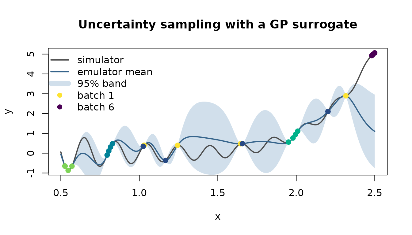

Figure 1: Active learning on the one-dimensional test function. Points show evaluated configurations, shaded by batch; the shaded region is the emulator’s 95% credible band after the final batch.

The components behind the interface

optimize_active() delegates the construction of its optimizer to the factory optimizer_al(), and every argument beyond the objective and the budget is in fact an argument of that factory. Constructing the optimizer explicitly makes the structure of the method visible and allows the same configured strategy to be reused, inspected, or embedded in larger experiments. The factory exposes three groups of choices: how the surrogate quantifies uncertainty, how candidates are generated, and how a batch is assembled from scored candidates.

tree_optimizer <- optimizer_al(
  learner = lrn("regr.rpart", minsplit = 2L, cp = 0),
  se_method = "bootstrap",
  n_bootstrap = 12L,
  batch_size = 2L,
  n_candidates = 200L,
  candidate_sampler = clx_sps("lhs"),
  multipoint_method = "greedy"
)

Surrogates and standard errors

Uncertainty sampling needs predictive standard errors, but many attractive regression models do not provide them natively. The se_method argument covers the three common situations:

"auto" uses the learner’s native "se" predict type when available, as with regr.km above, and falls back to "bootstrap" otherwise;
"bootstrap" wraps the learner in LearnerRegrBootstrapSE, which trains an ensemble of n_bootstrap models on bootstrap resamples and reports the ensemble mean and standard deviation;
"quantile" wraps a quantile-regression learner in LearnerRegrQuantileSE, which converts an inter-quantile range into a standard error.

Both wrappers are ordinary registered learners (lrn("regr.bootstrap_se"), lrn("regr.quantile_se")) and can be used outside active learning as well. In the configuration above, a regression tree – a model with no notion of predictive variance – becomes usable for uncertainty sampling through a twelve-member bootstrap ensemble.

Candidate generation

In each proposal round the acquisition function scores a finite set of n_candidates candidate points, and the candidate_sampler determines how this set is drawn from the domain. Samplers are SpaceSampler objects, collected in their own dictionary with the sugar constructors clx_sps() and clx_spss() (the clx_ prefix marks celecx sugar, in analogy to mlr3’s lrn() and msr()):

as.data.table(mlr_space_samplers)[, .(key, label)]
#> Key: <key>
#>                  key                            label
#>               <char>                           <char>
#> 1:             chain            Chained Space Sampler
#> 2:       conditional        Conditional Space Sampler
#> 3:               gsx                GSx Space Sampler
#> 4:            kmeans            K-Means Space Sampler
#> 5:          kmedoids          K-Medoids Space Sampler
#> 6:               lhs                LHS Space Sampler
#> 7: relational_kmeans Relational K-Means Space Sampler
#> 8:             sobol              Sobol Space Sampler
#> 9:           uniform            Uniform Space Sampler

The configuration above replaces the default uniform sampling by a Latin hypercube design, matching the common practice of ranking space-filling candidates by model uncertainty. Space-filling (lhs, sobol), geometric (gsx, the farthest-point strategy), and cluster-based (kmeans, kmedoids) samplers are interchangeable here, and the same objects also serve as initial-design generators.

Batch construction

When batch_size exceeds one, taking the top-scoring candidates (“greedy”) risks proposing near-duplicates, since neighbouring points have similar acquisition scores. The multipoint_method argument offers three sequential alternatives: "local_penalization" discounts scores near already-selected points (González et al., 2016), "diversity" adds an explicit distance-based diversity term, and "constant_liar" inserts pseudo-observations at selected points and rescores, following Ginsbourger et al. (2010). The tightly clustered same-batch points in Figure 1 show the phenomenon these methods address; for the small batches used in this vignette the greedy choice remains adequate, and we keep it.

Running a configured optimizer

A configured optimizer is passed to optimize_active() in place of the learner arguments. The run below repeats the experiment of Section 2 with the tree ensemble, a smaller batch size, and a larger budget; we will return to its archive in Section 5.

set.seed(2L)

result_tree <- optimize_active(
  objective = objective_1d,
  n_evals = 32L,
  optimizer = tree_optimizer
)

result_tree$instance
#> <SearchInstance>
#> * Objective: function
#> * Search space: 1 parameters
#> * Terminator: TerminatorEvals
#> * Evaluations: 32
#> * Batches: 15
#> * Terminated: TRUE
#> * Goal: learn

Under the hood: `OptimizerAL`

The factory itself only wires together components of the OptimizerAL class, and the same wiring can be written out explicitly. An OptimizerAL owns named surrogates and acquisition functions, an initial-design sampler, and a proposer that turns the current state into the next batch; proposers refer to surrogates and acquisition functions by their registry names. The following construction is, up to a technicality, what optimizer_al() assembled above (the factory additionally wraps the samplers so that the same optimizer serves both continuous domains and the finite pools of Section 4).

se_learner <- lrn("regr.bootstrap_se", learner = lrn("regr.rpart", minsplit = 2L, cp = 0))
se_learner$param_set$set_values(n_bootstrap = 12L)
se_learner$predict_type <- "se"

optimizer_manual <- OptimizerAL$new(
  proposer = ALProposerScore$new(
    acq_id = "sd",
    surrogate_id = "model",
    candidate_sampler = clx_sps("lhs"),
    n_candidates = 200L
  ),
  surrogates = list(
    model = mlr3mbo::SurrogateLearner$new(learner = se_learner, archive = NULL)
  ),
  acq_functions = list(sd = mlr3mbo::acqf("sd")),
  init_sampler = clx_sps("uniform"),
  result_assigner = ResultAssignerNull$new()
)
optimizer_manual$param_set$set_values(batch_size = 2L)

optimizer_manual
#> 
#> ── <OptimizerAL> - Active Learning ─────────────────────────────────────────────
#> • Parameters: batch_size=2, replace_samples=never, proposer.n_candidates=200,
#> proposer.acq_fit_scope=global, surrogate_model.catch_errors=TRUE,
#> surrogate_model.impute_method=random
#> • Parameter classes: <ParamDbl>, <ParamInt>, <ParamFct>, <ParamLgl>, and
#> <ParamUty>
#> • Properties: dependencies and single-crit
#> • Packages: bbotk, lhs, mlr3, celecx, and rpart

The print output shows how the components’ configuration surfaces in the optimizer’s parameter set under prefixes such as proposer. and surrogate_model.. This decomposition is also the extension interface: a new active-learning method is typically a new AcqFunction (possibly building on the distance-aware AcqFunctionDist family and an ALDistance from the mlr_al_distances dictionary, which includes a Gower distance for mixed continuous–categorical spaces) or a new ALProposer, wired exactly as above. The proposer classes shipped with the package – ALProposerScore, ALProposerSequentialScore, ALProposerSequentialReference, ALProposerPseudoLabel, and the round-robin ALProposerPortfolio – cover single-pass scoring, the sequential batch heuristics of Section 3.3, distance-based rescoring, pseudo-label updates, and method combination.

Active learning on a finite pool

So far, candidates could be placed anywhere in the domain. In many applications the choice is instead restricted to a finite pool of configurations: a library of prepared meshes or material compositions, a factorial catalogue of admissible settings, or – particularly relevant for method development – a dataset of already-computed simulations on which an active-learning strategy is to be replayed as if the outcomes were still unknown. Pool-based active learning is also where the best-known methods from the regression active-learning literature are formulated.

Pool objectives

ObjectiveDataset wraps a pre-evaluated table as an objective that evaluates by lookup and rejects configurations outside the table. We discretize the simulator of Section 2 into a pool of 101 candidate runs:

pool <- data.table(x = seq(0.5, 2.5, length.out = 101L))
pool[, y := simulator_1d(x)]

objective_pool <- ObjectiveDataset$new(
  dataset = pool,
  domain = ps(x = p_dbl(lower = 0.5, upper = 2.5)),
  codomain = ps(y = p_dbl(tags = "learn"))
)

Such objectives carry the property "pool_restricted", and OptimizerAL reacts to it: initial designs and candidate sets are then drawn from the not-yet-evaluated pool rows rather than from the continuous domain, so the optimizers of the previous sections work unchanged. (By default an evaluated pool row is never proposed again; the optimizer’s replace_samples parameter relaxes this.) For on-demand evaluation restricted to a candidate list, ObjectivePoolRFun and ObjectivePoolWrapper provide the same behaviour around a live function.

Named methods from the literature

optimizer_pool_al() constructs the standard pool-based methods, again as OptimizerAL wirings:

`method`	Strategy	Reference	Learner used
`"random"`	uniform random sampling	–	none
`"gsx"`	greedy sampling in input space	Wu et al. (2019)	none
`"gsy"`	greedy sampling in output space	Wu et al. (2019)	predictions
`"igs"`	improved greedy sampling, input $\times$ output	Wu et al. (2019)	predictions
`"qbc"`	query by committee via bootstrap disagreement	Seung et al. (1992); RayChaudhuri and Hamey (1995)	committee
`"ideal"`	inverse-distance weighted residuals plus exploration	Bemporad (2023)	predictions

GSx spreads evaluations by always taking the pool point farthest from the evaluated set; it needs no model at all. GSy transfers the same greedy logic to the response scale, preferring candidates whose predicted output differs most from all observed outputs, and iGS combines both distances multiplicatively. QBC queries where a bootstrap committee of models disagrees most, and IDEAL scores candidates by inverse-distance-weighted residuals together with a geometric exploration term whose weight is set by delta. Each method comes with its customary initialization, which init_method can override ("gsx", "random", or "kmeans", the latter selecting cluster-representative pool points).

Comparing selection behaviour

We run four of the methods on the pool with identical budgets: sixteen evaluations, of which the first four form the initial design. The model-based methods use the Gaussian process as their learner.

pool_optimizers <- list(
  random = optimizer_pool_al("random", n_init = 4L),
  gsx = optimizer_pool_al("gsx", n_init = 4L),
  igs = optimizer_pool_al("igs", learner = km_learner(), n_init = 4L),
  ideal = optimizer_pool_al("ideal", learner = km_learner(), n_init = 4L)
)

pool_results <- list()
for (method in names(pool_optimizers)) {
  set.seed(4L)
  pool_results[[method]] <- optimize_active(
    objective = objective_pool,
    n_evals = 16L,
    optimizer = pool_optimizers[[method]]
  )
}

Figure 2 shows which pool points each method selected, numbered by evaluation order. Random sampling scatters without regard to geometry, and GSx produces a near-equispaced space-filling sequence. The model-based methods behave differently: iGS and IDEAL both shift effort towards the right half of the domain, where the steep trend produces large output differences and large residuals, respectively.

plot_pool_run <- function(result, title) {
  archive <- result$instance$archive$data
  order_colors <- hcl.colors(nrow(archive), "Viridis", rev = TRUE)
  plot(pool$x, pool$y, type = "l", col = "grey60",
    xlab = "x", ylab = "y", main = title)
  points(pool$x, pool$y, pch = 16, cex = 0.35, col = "grey75")
  points(archive$x, archive$y, pch = 19, cex = 1.1, col = order_colors)
  text(archive$x, archive$y, labels = seq_len(nrow(archive)), pos = 3,
    cex = 0.7, offset = 0.35)
}

old_par <- par(mfrow = c(2, 2), mar = c(4, 4, 2.5, 1))
for (method in names(pool_results)) {
  plot_pool_run(pool_results[[method]], method)
}

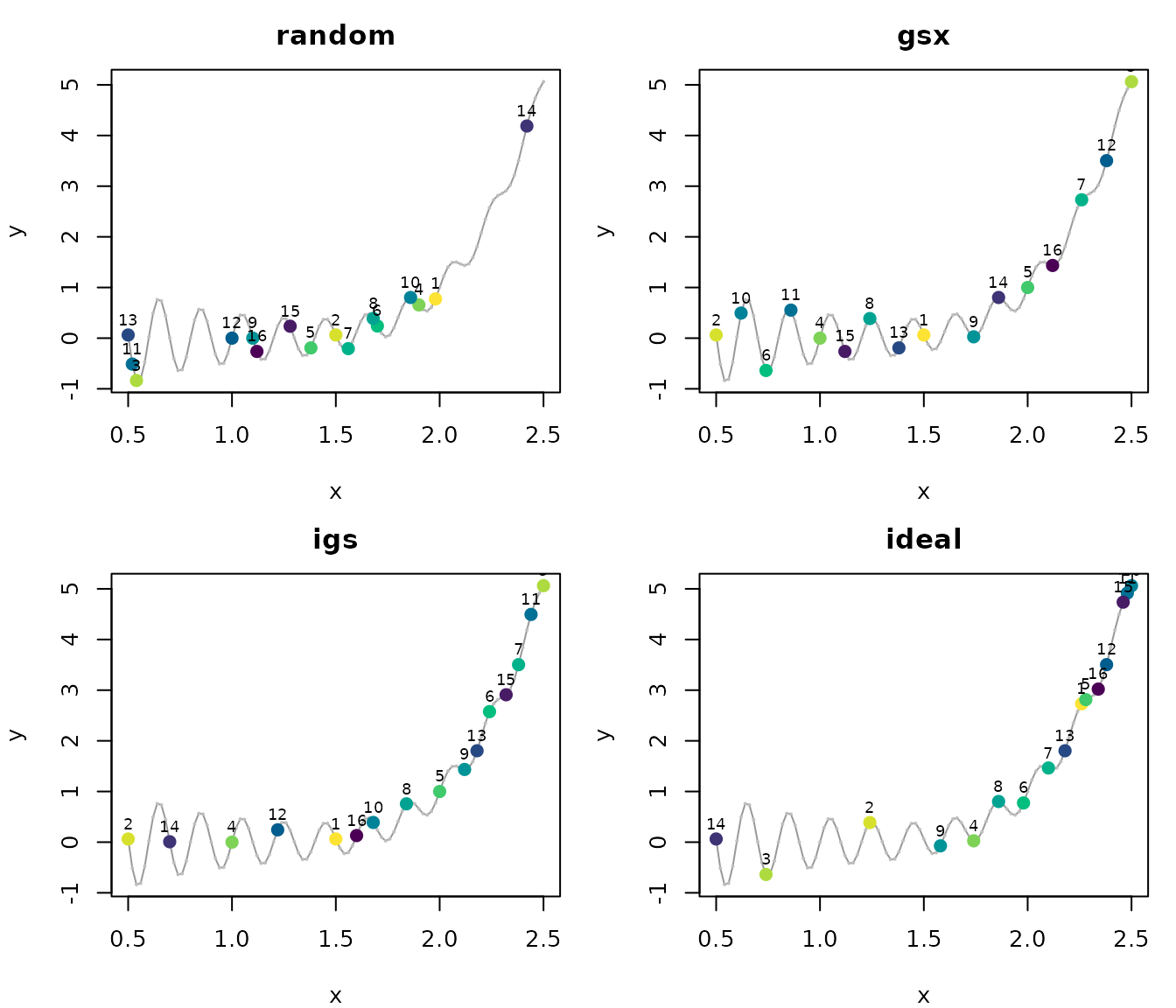
Figure 2: Selection behaviour of four pool-based methods on the same candidate pool. Numbers give the evaluation order; the first four points are the initial design.

par(old_par)

Which of these strategies actually learns fastest cannot be read off a selection plot; it is a question about the resulting model quality over time. That question leads directly to the second half of the package.

Learning curves

An active-learning run does not usually end because the model has become good enough; it ends because the budget is exhausted. The economically relevant question during a campaign is prospective: given how quality has developed so far, how many further batches will be needed to reach the target? The remainder of this vignette develops the celecx answer on a single running example. The first step, taken in this section, is to make “quality so far” a concrete object: one surrogate-performance value per evaluated batch, recorded during or after the run.

A two-dimensional simulation campaign

The running example is a smooth response surface over $[0, 1]^2$, two broad overlapping rises on a mild trend, standing in for, say, a simulated process yield over two design parameters. We aim for an emulator whose mean absolute error, over the whole design region, falls below a set target.

simulator_2d <- function(x1, x2) {
  1000 * (exp(-2 * ((x1 - 0.35)^2 + (x2 - 0.6)^2)) +
    0.5 * exp(-3 * ((x1 - 0.85)^2 + (x2 - 0.15)^2)) +
    0.3 * x1)
}

objective_2d <- ObjectiveRFun$new(
  fun = function(xs) list(y = simulator_2d(xs$x1, xs$x2)),
  domain = ps(x1 = p_dbl(0, 1), x2 = p_dbl(0, 1)),
  codomain = ps(y = p_dbl(tags = "learn"))
)

Measuring surrogate quality requires a held-out regression task on which the surrogate is scored. In a synthetic study we can afford a dense grid of true function values; in a real campaign the same role is played by whatever reference data are available, for example a reserved set of past simulator runs. The held-out task is an ordinary mlr3 regression task:

test_grid <- CJ(x1 = seq(0, 1, length.out = 24L), x2 = seq(0, 1, length.out = 24L))
test_grid[, y := simulator_2d(x1, x2)]
test_task_2d <- as_task_regr(test_grid, target = "y", id = "held_out_2d")

Recording the curve online

CallbackSurrogatePerformance hooks into the run and, after every evaluated batch including the initial design, scores a named surrogate of the optimizer on the held-out task. The callback is retrieved from the callback dictionary via clbk(); surrogate_id = "model" refers to the surrogate registry of optimizer_al(), and any list of regression measures can be tracked.

progress <- clbk("celecx.surrogate_performance",
  surrogate_id = "model",
  task = test_task_2d,
  measures = list(mae = msr("regr.mae"), rsq = msr("regr.rsq"))
)

set.seed(3L)

result_campaign <- optimize_active(
  objective = objective_2d,
  n_evals = 60L,
  learner = km_learner(),
  se_method = "auto",
  batch_size = 4L,
  n_candidates = 400L,
  callbacks = list(progress)
)

The campaign evaluated an initial design of eight points ($4 \cdot d$ with $d = 2$) followed by thirteen batches of four simulator runs each. The callback accumulated one row per batch:

progress$data[, .(batch_nr, n_evals, mae = signif(mae, 3), rsq = round(rsq, 4))]
#>     batch_nr n_evals     mae    rsq
#>        <int>   <int>   <num>  <num>
#>  1:        1       8 112.000 0.2741
#>  2:        2      12  16.300 0.9844
#>  3:        3      16   8.690 0.9961
#>  4:        4      20   4.120 0.9987
#>  5:        5      24   2.930 0.9992
#>  6:        6      28   0.817 1.0000
#>  7:        7      32   0.961 1.0000
#>  8:        8      36   0.714 1.0000
#>  9:        9      40   0.447 1.0000
#> 10:       10      44   0.242 1.0000
#> 11:       11      48   0.265 1.0000
#> 12:       12      52   0.175 1.0000
#> 13:       13      56   0.146 1.0000
#> 14:       14      60   0.108 1.0000

The two measures tell complementary stories. $R^2$ saturates almost immediately – it exceeds $0.999$ within a handful of batches – while the mean absolute error keeps falling by orders of magnitude long after that. For emulator construction, where pointwise accuracy matters, the absolute error is the more informative quantity, and we use the MAE curve from here on. Figure 3 shows the campaign. The design ends up close to space-filling – for a surface this smooth, predictive uncertainty is governed mainly by data density – and the error decays over roughly three orders of magnitude, approximately linearly on the logarithmic scale with a gradually flattening slope.

archive_campaign <- result_campaign$instance$archive$data
n_campaign_batches <- max(archive_campaign$batch_nr)
campaign_colors <- hcl.colors(n_campaign_batches, "Viridis", rev = TRUE)

old_par <- par(mfrow = c(1, 2), mar = c(4, 4, 2.5, 1))
x1_seq <- seq(0, 1, length.out = 60L)
x2_seq <- seq(0, 1, length.out = 60L)
contour(x1_seq, x2_seq, outer(x1_seq, x2_seq, simulator_2d),
  nlevels = 10, col = "grey60", xlab = "x1", ylab = "x2", main = "Design")
points(archive_campaign$x1, archive_campaign$x2, pch = 19, cex = 0.8,
  col = campaign_colors[archive_campaign$batch_nr])
plot(progress$data$batch_nr, progress$data$mae, log = "y", type = "b", pch = 19,
  xlab = "batch", ylab = "held-out MAE", main = "Learning curve")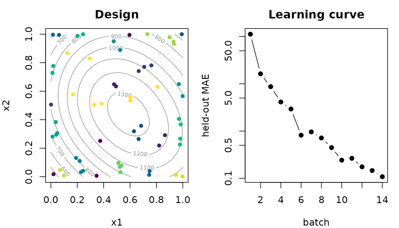

Figure 3: The two-dimensional campaign. Left: simulator contours with the evaluated design, shaded by batch. Right: held-out mean absolute error of the emulator after each batch.

par(old_par)

The learning-curve task

The callback converts its records into a TaskLCE, the task type under which learning curves become mlr3 data. Two arguments matter here. The measure argument selects which tracked measure becomes the prediction target. The link argument declares the scale on which forecasting models should represent the curve and its uncertainty: a MAE is positive and decays multiplicatively, so we model it on the logarithmic scale, which also guarantees that predictive distributions respect the lower bound of zero. The helper lce_link_from_range() suggests a link from a measure’s theoretical range ("log" for losses on $(0, \infty)$, "logit" for scores on $(0, 1)$, "identity" otherwise):

lce_link_from_range(msr("regr.mae")$range)
#> [1] "log"

task_campaign <- progress$task(measure = "mae", link = "log", id = "campaign")
task_campaign
#> 
#> ── <TaskLCE> (60x2) ────────────────────────────────────────────────────────────
#> • Target: mae
#> • Properties: -
#> • Features (1):
#>   • int (1): batch_nr
#> • Archive features: x1 and x2
#> • Archive targets: y

The task has one row per archive evaluation, not per batch; all rows of a batch share that batch’s performance value. Its single feature is the batch number, which is all that a forecasting model needs at prediction time – forecasting the curve at future batches must not require knowing which points those batches will contain.

head(task_campaign$data(), 3L)
#>         mae batch_nr
#>       <num>    <int>
#> 1: 112.0766        1
#> 2: 112.0766        1
#> 3: 112.0766        1

The archive’s input and output columns are nevertheless carried along, under the dedicated column roles archive_x and archive_y (accessible via $archive_x_data() and $archive_y_data()), because advanced extrapolators inspect the archive during training. For the same reason the task stores run provenance: the search space and codomain of the originating run, the regression measure that produced the target (task_campaign$measure), the candidate pool for pool-based runs (task_campaign$pool, NULL here), and the link name (task_campaign$link). Section 6.3 shows a forecaster that consumes all of it.

Reconstructing curves offline

Attaching the callback requires having thought of it before the run. replay_surrogate_performance() removes that requirement: given a finished archive, it refits a surrogate on each batch prefix, scores it on the held-out task, and returns the same kind of TaskLCE. Beyond rescuing untracked runs, replay decouples the curve from the run in two useful ways: the replayed surrogate need not be the one that drove the design, so several emulator choices can be scored on the same trace, and runs whose strategy maintained no model at all – GSx or random sampling, say – still yield learning curves.

The tree-ensemble run of Section 3 was not tracked; we reconstruct its curve now, scoring against a dense held-out grid of the one-dimensional function.

dense_1d <- data.table(x = seq(0.5, 2.5, length.out = 201L))
dense_1d[, y := simulator_1d(x)]
test_task_1d <- as_task_regr(dense_1d, target = "y", id = "held_out_1d")

tree_se_learner <- lrn("regr.bootstrap_se", learner = lrn("regr.rpart", minsplit = 2L, cp = 0))
tree_se_learner$param_set$set_values(n_bootstrap = 12L)
tree_se_learner$predict_type <- "se"

set.seed(21L)
task_tree <- replay_surrogate_performance(
  archive = result_tree$instance$archive,
  learner = tree_se_learner,
  task = test_task_1d,
  measures = list(mae = msr("regr.mae")),
  link = "log",
  id = "surrogate_1d"
)

tree_curve <- unique(task_tree$data()[, .(batch_nr, mae)])
plot(tree_curve$batch_nr, tree_curve$mae, log = "y", type = "b", pch = 19,
  xlab = "batch", ylab = "held-out MAE", main = "Replayed learning curve (tree ensemble)")

Figure 4: Learning curve of the Section 3 tree-ensemble run, reconstructed offline by replaying its archive.

This curve looks qualitatively different from the campaign’s: after early gains it flattens out near a plateau, the bias floor of a piecewise-constant model on a smooth function. We keep both tasks; their contrast becomes instructive in Section 7.

Extrapolating learning curves

A TaskLCE is a task, so extrapolation methods are learners: they train on the observed prefix of a curve and predict performance at future batch numbers. celecx registers them under the lce. prefix in the standard learner dictionary:

grep("^lce\\.", mlr_learners$keys(), value = TRUE)
#>  [1] "lce.bootstrap"              "lce.conformal"             
#>  [3] "lce.featureless"            "lce.gam"                   
#>  [5] "lce.isotonic"               "lce.parametric_exponential"
#>  [7] "lce.parametric_log"         "lce.parametric_logistic"   
#>  [9] "lce.parametric_power_law"   "lce.rolling_slope"         
#> [11] "lce.simulate"               "lce.spline_monotone"

The families are, in increasing order of structure: featureless baselines (lce.featureless predicts the best, last, or average observed value forever); a local trend baseline (lce.rolling_slope extends a straight line fit to the most recent batches); parametric curve families from the learning-curve literature (Viering and Loog, 2023) – lce.parametric_exponential fits $f(b) = c + a e^{-kb}$, lce.parametric_power_law fits $f(b) = c + a b^{-k}$, and lce.parametric_log and lce.parametric_logistic fit logarithmic and sigmoidal shapes; monotone nonparametric fits (lce.isotonic, and lce.spline_monotone if the scam package is installed), which impose the shape constraint without committing to a family; wrappers that endow a base learner with distributional predictions (lce.bootstrap, lce.conformal); and the forward-simulation learner lce.simulate, treated in Section 6.3. All of them fit the curve on the task’s link scale, here the log scale.

Forecasting mid-campaign

To use the campaign as an honest test bed, we place ourselves at batch 8 – roughly the campaign’s midpoint, MAE just above $0.7$ – and forecast from there, keeping the remaining batches for comparison. Restricting a task to a batch prefix is a matter of filtering rows:

forecast_batch <- 8L
task_past <- task_campaign$clone(deep = TRUE)
task_past$filter(task_past$row_ids[task_past$batch_nrs <= forecast_batch])

realized <- unique(task_campaign$data()[, .(batch_nr, mae)])

We train four point forecasters on the prefix and predict the full range of batches. Prediction at new batch numbers uses the standard predict_newdata() mechanism; note that batch_nr must be supplied as an integer column.

point_learners <- list(
  featureless = lrn("lce.featureless"),
  rolling_slope = lrn("lce.rolling_slope"),
  exponential = lrn("lce.parametric_exponential"),
  power_law = lrn("lce.parametric_power_law")
)

batch_grid <- data.table(batch_nr = 1:16L)
point_forecasts <- sapply(point_learners, function(learner) {
  learner$train(task_past)
  learner$predict_newdata(batch_grid)$response
})

forecast_colors <- hcl.colors(5, "Dark 3")[1:4]
matplot(batch_grid$batch_nr, point_forecasts, log = "y", type = "l", lty = 1,
  lwd = 2, col = forecast_colors, ylim = range(realized$mae, point_forecasts),
  xlab = "batch", ylab = "held-out MAE",
  main = "Extrapolating the campaign curve")
abline(v = forecast_batch + 0.5, lty = 3, col = "grey50")
points(realized[batch_nr <= forecast_batch], pch = 19)
points(realized[batch_nr > forecast_batch], pch = 1)
legend("bottomleft", legend = colnames(point_forecasts), col = forecast_colors,
  lwd = 2, bty = "n")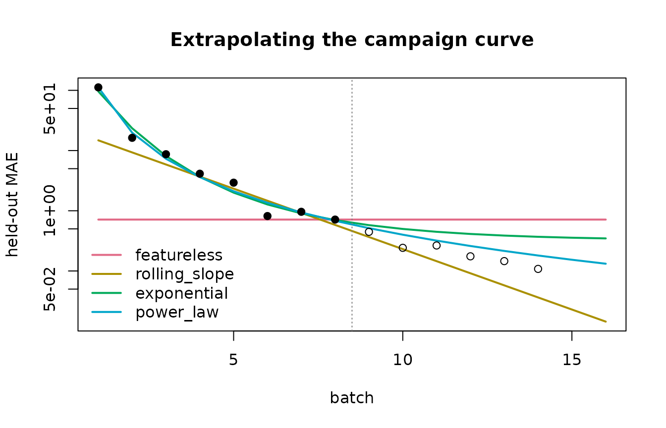

Figure 5: Point forecasts from batch 8. Filled circles are the batches available to the forecasters, open circles the realized continuation.

The four methods embody different beliefs about what comes next, and the figure makes the differences concrete. The featureless baseline (predicting the best value seen so far) denies any further progress. The rolling slope continues the recent log-linear trend indefinitely and therefore predicts the fastest progress. The two parametric families interpolate between these extremes: both admit deceleration, but the exponential’s fixed asymptote, estimated from an early prefix, is pessimistic about the later batches, while the power law’s slower decay tracks the realized continuation more closely here. None of this is specific to the example – which family extrapolates best depends on the curve, which is exactly why Section 7 treats the choice as an empirical model-selection problem.

Distributional forecasts

Point forecasts are rarely enough: a stopping decision needs to know how certain the forecast is. LearnerLCE objects therefore support distributional predict types beyond "response":

"se" adds two standard errors on the link scale: se, the total predictive standard deviation of a future realized curve value, and se_epistemic, the narrower uncertainty of the mean curve itself. The distinction matters because a realized batch value scatters around the mean curve with residual noise even if the curve were known exactly.
"quantiles" returns predictive quantiles on the natural scale.
"samples" returns joint sample paths, which preserve the dependence between future batches.
"target_reached" returns, per batch, the probability that a configurable target has been reached.

The parametric learners derive se analytically from the curve fit. A more assumption-averse route is the residual-bootstrap wrapper lce.bootstrap, which refits its base learner on many resampled versions of the curve and reads uncertainty off the spread of the refits; being sample-based, it supports all predict types including joint paths. We wrap the power law:

forecaster <- lrn("lce.bootstrap",
  learner = lrn("lce.parametric_power_law"),
  n_bootstrap = 100L, seed = 1L)
forecaster$predict_type <- "se"
forecaster$train(task_past)

prediction_se <- as.data.table(forecaster$predict_newdata(batch_grid))
tail(cbind(batch_grid, prediction_se[, .(response = signif(response, 3),
  se = signif(se, 3), se_epistemic = signif(se_epistemic, 3))]), 4L)
#>    batch_nr response    se se_epistemic
#>       <int>    <num> <num>        <num>
#> 1:       13    0.243 0.367        0.264
#> 2:       14    0.208 0.383        0.286
#> 3:       15    0.179 0.399        0.307
#> 4:       16    0.156 0.415        0.328

On the log link, a central 90% band around the predictive median is obtained as $\text{response} \cdot \exp(\pm z_{0.95} \cdot \text{se})$. Figure 6 shows the epistemic and total bands together with a handful of joint sample paths, and the realized continuation for reference.

z90 <- qnorm(0.95)
forecaster$predict_type <- "samples"
future_grid <- data.table(batch_nr = (forecast_batch + 1L):16L)
sample_paths <- forecaster$predict_newdata(future_grid)$samples

plot(realized$batch_nr, realized$mae, log = "y", type = "n",
  xlim = c(1, 16), ylim = range(realized$mae) * c(0.2, 2),
  xlab = "batch", ylab = "held-out MAE", main = "Bootstrap power-law forecast")
polygon(c(batch_grid$batch_nr, rev(batch_grid$batch_nr)),
  c(prediction_se$response * exp(z90 * prediction_se$se),
    rev(prediction_se$response * exp(-z90 * prediction_se$se))),
  col = adjustcolor("darkorange", alpha.f = 0.15), border = NA)
polygon(c(batch_grid$batch_nr, rev(batch_grid$batch_nr)),
  c(prediction_se$response * exp(z90 * prediction_se$se_epistemic),
    rev(prediction_se$response * exp(-z90 * prediction_se$se_epistemic))),
  col = adjustcolor("darkorange", alpha.f = 0.35), border = NA)
matlines(future_grid$batch_nr, sample_paths[, 1:15],
  lty = 1, lwd = 0.5, col = adjustcolor("grey30", alpha.f = 0.35))
lines(batch_grid$batch_nr, prediction_se$response, lwd = 2, col = "darkorange3")
abline(v = forecast_batch + 0.5, lty = 3, col = "grey50")
points(realized[batch_nr <= forecast_batch], pch = 19)
points(realized[batch_nr > forecast_batch], pch = 1)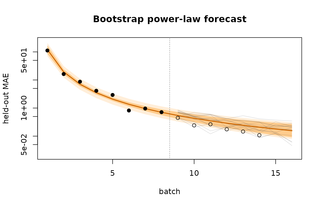

Figure 6: Distributional forecast of the bootstrap power law from batch 8: central 90% bands from the epistemic (dark) and total (light) standard errors, thin lines showing 15 joint sample paths of the realized future curve, and the realized continuation (open circles).

The alternative wrapper lce.conformal calibrates a constant-width band on a hold-out suffix of the training batches by split-conformal inference, trading the Gaussian working assumption for finite-sample marginal coverage at its configured level.

Policy-aware forecasting by forward simulation

All learners so far look only at the shape of the observed curve. lce.simulate uses the run provenance stored in the task instead: at training time it fits an oracle regression model on the archive’s input–output pairs, and at prediction time it re-runs the configured active-learning optimizer forward from the training archive, using the oracle in place of the simulator, and scores the simulated surrogate after each simulated batch. Its forecast is thus not a curve family but the outcome of actually executing the acquisition policy on the best available stand-in for the truth – connecting the forecasting half of the package back to the active-learning half. The optimizer configuration and the oracle are supplied at construction; measure, search space, and pool are read from the task.

sim_forecaster <- lrn("lce.simulate",
  optimizer = optimizer_al(
    learner = km_learner(),
    se_method = "auto",
    batch_size = 4L,
    n_candidates = 400L
  ),
  oracle_learner = km_learner(),
  n_restarts = 3L,
  seed = 1L
)
sim_forecaster$train(task_past)
sim_prediction <- sim_forecaster$predict_newdata(future_grid)

sim_table <- data.table(
  batch_nr = future_grid$batch_nr,
  simulated = signif(sim_prediction$response, 3)
)
merge(sim_table, realized[, .(batch_nr, realized = signif(mae, 3))],
  by = "batch_nr", all.x = TRUE)
#> Key: <batch_nr>
#>    batch_nr simulated realized
#>       <int>     <num>    <num>
#> 1:        9    0.1510    0.447
#> 2:       10    0.1380    0.242
#> 3:       11    0.0558    0.265
#> 4:       12    0.0637    0.175
#> 5:       13    0.0576    0.146
#> 6:       14    0.0427    0.108
#> 7:       15    0.0394       NA
#> 8:       16    0.0206       NA

The simulated curve reproduces the shape of the continuation but sits below the realized values. This bias is inherent to the construction: the forecast scores the simulated surrogate against the oracle’s own predictions, and the oracle – fit on 36 points – is smoother than the true response surface, so the simulated problem is easier than the real one. The simulation forecast is therefore most valuable where the curve-fitting learners are blind by construction: it reacts to the acquisition policy, the batch size, and the candidate budget, and it produces joint sample paths (one per restart) whose spread reflects the stochasticity of the policy itself.

Evaluating extrapolators

Which forecaster should be trusted for a given campaign? Since extrapolators are learners, this is a resampling question, answered with the standard mlr3 tools. Two ingredients are specific to learning curves: the resampling scheme and the measures.

For resampling, random train–test splits would leak future batches into training. ResamplingLCE (rsmp("lce.expanding_cv")) instead splits by whole batches in temporal order: each fold trains on all batches up to a moving cut-off and tests on the following horizon batches, with the cut-off advancing by step_size between folds. The first cut-off, min_train_batches, has deliberately no default, since results are sensitive to how much history the forecasters see; it must also respect the learners’ own minima (the parametric families need a handful of batches, lce.spline_monotone needs five).

The registered measures score per-batch forecasts:

grep("^lce\\.", mlr_measures$keys(), value = TRUE)
#> [1] "lce.coverage"       "lce.crps"           "lce.interval_score"
#> [4] "lce.mae"            "lce.mse"            "lce.pinball"       
#> [7] "lce.reach_brier"    "lce.rmse"

lce.mae, lce.mse, and lce.rmse are point-forecast losses on the natural scale. The distributional measures read the Gaussian-on-link predictive carried by the "se" predict type: lce.crps is the closed-form continuous ranked probability score (a proper score, our headline distributional criterion), lce.coverage and lce.interval_score assess central prediction intervals, lce.pinball scores predicted quantiles, and lce.reach_brier evaluates the predicted probability of having reached a target – the decision-oriented criterion matching Section 8.

We benchmark five forecasters on both learning-curve tasks, with folds forecasting two batches ahead:

bench_learners <- list(
  lrn("lce.featureless"),
  lrn("lce.rolling_slope", window = 4L),
  lrn("lce.parametric_exponential"),
  lrn("lce.parametric_power_law"),
  lrn("lce.bootstrap", learner = lrn("lce.parametric_power_law"),
    n_bootstrap = 100L, seed = 1L)
)
for (learner in bench_learners) {
  learner$predict_type <- "se"
}

resampling <- rsmp("lce.expanding_cv",
  min_train_batches = 5L, horizon = 2L, step_size = 1L)

set.seed(5L)
benchmark_result <- benchmark(benchmark_grid(
  tasks = list(task_campaign, task_tree),
  learners = bench_learners,
  resamplings = resampling
))

aggregated <- benchmark_result$aggregate(
  list(msr("lce.mae"), msr("lce.crps"), msr("lce.coverage"))
)
aggregated[, .(task_id, learner_id,
  lce.mae = signif(lce.mae, 3),
  lce.crps = round(lce.crps, 3),
  lce.coverage = round(lce.coverage, 2))]
#>          task_id                             learner_id lce.mae lce.crps
#>           <char>                                 <char>   <num>    <num>
#>  1:     campaign                        lce.featureless 0.39200    0.522
#>  2:     campaign                      lce.rolling_slope 0.17700    0.294
#>  3:     campaign             lce.parametric_exponential 0.28900    0.293
#>  4:     campaign               lce.parametric_power_law 0.18900    0.210
#>  5:     campaign lce.bootstrap.lce.parametric_power_law 0.19200    0.234
#>  6: surrogate_1d                        lce.featureless 0.00739    0.062
#>  7: surrogate_1d                      lce.rolling_slope 0.01830    0.051
#>  8: surrogate_1d             lce.parametric_exponential 0.01570    0.046
#>  9: surrogate_1d               lce.parametric_power_law 0.01430    0.037
#> 10: surrogate_1d lce.bootstrap.lce.parametric_power_law 0.01230    0.031
#>     lce.coverage
#>            <num>
#>  1:         1.00
#>  2:         0.75
#>  3:         0.88
#>  4:         0.88
#>  5:         0.75
#>  6:         1.00
#>  7:         0.83
#>  8:         0.89
#>  9:         1.00
#> 10:         1.00

The two tasks reward different beliefs, as anticipated in Section 5.4. On the steadily improving campaign curve, the trend-following forecasters (rolling slope, power law) clearly beat the featureless baseline at both point and distributional accuracy. On the plateaued tree curve the ranking inverts for point forecasts: predicting the best value seen so far is hard to beat once a curve has flattened, and the flexible extrapolators pay for occasionally chasing noise – although the distributional scores still favour the calibrated forecasters. The practical reading is that no family dominates across traces, and that the forecaster feeding a costly stopping decision should first be validated on the trace types it will face; the benchmark above is precisely that validation, in miniature. (With a single task and learner, resample() replaces benchmark() in the usual mlr3 manner.)

From forecasts to decisions: batches to target

The question from the beginning of Section 5 – how many further batches? – is answered by lce_batches_to_target(). Given a trained forecaster, a future batch grid, and a performance target, it converts the per-batch predictive distributions into a distribution over the batch at which the target is first reached, reporting its quantiles, the full CDF over the grid, and the probability that the grid never reaches the target at all. The optimization direction (here: lower is better) is read from the measure stored in the training task.

Two crossing semantics are available. crossing = "expected" asks when the mean curve passes the target – the de-noised notion appropriate for “when will the model truly be good enough”, computed from se_epistemic. crossing = "observed" asks when the realized, noisy curve first dips below the target, the literal stopping time of a run that halts on its progress plot; being a first-passage property of a correlated sequence, it requires joint sample paths and hence a sample-based learner. The observed crossing necessarily happens no later in distribution than the expected one, since noise can dip below the target early.

We set the target at a MAE of $0.2$ and forecast from batch 8, using the bootstrap power law of Section 6.2 and, for contrast, a bootstrap around the rolling slope:

mae_target <- 0.2

b2t_power_law <- lce_batches_to_target(forecaster,
  batch_grid = 9:24L, target = mae_target, crossing = "expected")
b2t_power_law_observed <- lce_batches_to_target(forecaster,
  batch_grid = 9:24L, target = mae_target, crossing = "observed")

slope_forecaster <- lrn("lce.bootstrap",
  learner = lrn("lce.rolling_slope"), n_bootstrap = 100L, seed = 1L)
slope_forecaster$train(task_past)
b2t_slope <- lce_batches_to_target(slope_forecaster,
  batch_grid = 9:24L, target = mae_target, crossing = "expected")

rbind(
  data.table(forecaster = "power law (expected)", t(b2t_power_law$quantiles),
    p_never = round(b2t_power_law$p_never, 3)),
  data.table(forecaster = "power law (observed)", t(b2t_power_law_observed$quantiles),
    p_never = round(b2t_power_law_observed$p_never, 3)),
  data.table(forecaster = "rolling slope (expected)", t(b2t_slope$quantiles),
    p_never = round(b2t_slope$p_never, 3))
)
#>                  forecaster  q0.1  q0.5  q0.9 p_never
#>                      <char> <num> <num> <num>   <num>
#> 1:     power law (expected)    13    15    18    0.01
#> 2:     power law (observed)    12    14    18    0.01
#> 3: rolling slope (expected)     9    12    21    0.08

In the campaign that actually continued, the target was first reached in batch 12.

plot(b2t_power_law$grid$batch, b2t_power_law$grid$cdf, type = "s", lwd = 2,
  col = "darkorange3", ylim = c(0, 1), xlab = "batch",
  ylab = "P(target reached by batch)", main = "Batches-to-target forecast")
lines(b2t_slope$grid$batch, b2t_slope$grid$cdf, type = "s", lwd = 2,
  col = "steelblue4")
abline(v = realized[mae <= mae_target, min(batch_nr)], lty = 2, col = "grey40")
abline(h = c(0.1, 0.5, 0.9), lty = 3, col = "grey75")
legend("topleft", legend = c("bootstrap power law", "bootstrap rolling slope"),
  col = c("darkorange3", "steelblue4"), lwd = 2, bty = "n")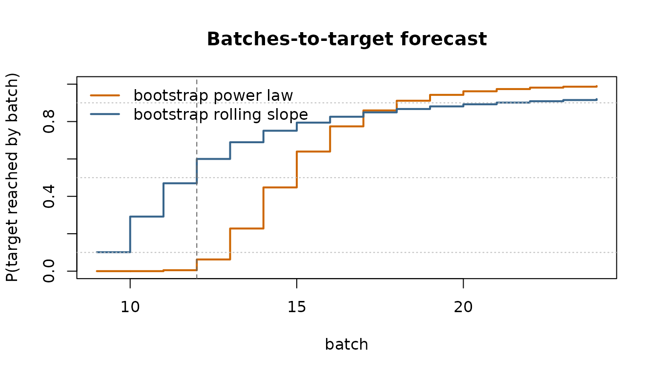

Figure 7: Batches-to-target forecasts made at batch 8 for a target MAE of 0.2: probability that the target has been reached, per batch, under two forecasters. The vertical line marks the batch in which the continued campaign actually reached the target.

The two forecasters bracket the realized outcome: the rolling slope, extrapolating the recent trend, gives a median of about batch 12 with wide uncertainty and some probability mass on “not within the grid”, while the more cautious power law places its median around batch 15, two to three batches after the realized crossing and with its lower decile just missing it. This residual disagreement is the honest state of knowledge at batch 8, and the benchmark of Section 7 is the tool for deciding which of the two to weight more heavily. Either way the forecast is directly actionable: multiplying batches by the batch size of four converts the answer into simulator evaluations, which can be set against the cost of computing them and the value of reaching the target.

Concluding remarks

The path taken by this vignette is the intended shape of a celecx analysis. An objective wraps the expensive simulator (Section 2), an OptimizerAL – assembled by a factory or by hand – runs batch-sequential active learning on it (Sections 2 to 4), a callback or an offline replay condenses the run into a TaskLCE (Section 5), learning-curve learners fit and extrapolate that task with calibrated uncertainty (Section 6), resampling and benchmarking select among them (Section 7), and lce_batches_to_target() turns the selected forecaster into a stopping decision (Section 8). Because every stage speaks the mlr3 language, each of them can be swapped out or studied in isolation: active-learning strategies are optimizers, emulators and their uncertainty wrappers are regression learners, learning curves are tasks, and extrapolators are learners with measures and resampling schemes of their own.

Several parts of the package did not fit into this introduction. Among the surrogates, wrappers for further Gaussian-process backends (regr.gpfit, regr.hetgp, regr.tgp, regr.deepgp) cover heteroscedastic and nonstationary emulation. Among the pool tools, ObjectivePoolRFun and ObjectivePoolWrapper restrict live objectives to candidate lists, and the ALDistance dictionary (clx_ald()) underlying the distance-based acquisition functions extends them to mixed continuous–categorical spaces. Among the forecasters, lce.parametric_log, lce.parametric_logistic, lce.isotonic, and lce.spline_monotone provide further curve shapes, the "quantiles" and "target_reached" predict types expose the predictive distribution in other formats, and the measures lce.pinball, lce.interval_score, and lce.reach_brier score them. The help pages of the classes encountered above document these variations, and each dictionary (mlr_space_samplers, mlr_al_distances, and the lce. entries of mlr_learners and mlr_measures) can be listed and explored in the usual mlr3 fashion.

References

Bemporad, A. (2023). Active learning for regression by inverse distance weighting. Information Sciences, 626, 275–292.

Ginsbourger, D., Le Riche, R., and Carraro, L. (2010). Kriging is well-suited to parallelize optimization. In Computational Intelligence in Expensive Optimization Problems, 131–162. Springer.

González, J., Dai, Z., Hennig, P., and Lawrence, N. (2016). Batch Bayesian optimization via local penalization. In Proceedings of AISTATS 2016, 648–657.

Gramacy, R. B. (2020). Surrogates: Gaussian Process Modeling, Design, and Optimization for the Applied Sciences. CRC Press.

Gramacy, R. B. and Lee, H. K. H. (2012). Cases for the nugget in modeling computer experiments. Statistics and Computing, 22(3), 713–722.

RayChaudhuri, T. and Hamey, L. G. C. (1995). Minimisation of data collection by active learning. In Proceedings of ICNN 1995, 1338–1341.

Roustant, O., Ginsbourger, D., and Deville, Y. (2012). DiceKriging, DiceOptim: Two R packages for the analysis of computer experiments by kriging-based metamodeling and optimization. Journal of Statistical Software, 51(1), 1–55.

Sacks, J., Welch, W. J., Mitchell, T. J., and Wynn, H. P. (1989). Design and analysis of computer experiments. Statistical Science, 4(4), 409–423.

Santner, T. J., Williams, B. J., and Notz, W. I. (2018). The Design and Analysis of Computer Experiments. Second edition. Springer.

Settles, B. (2009). Active learning literature survey. Computer Sciences Technical Report 1648, University of Wisconsin–Madison.

Seung, H. S., Opper, M., and Sompolinsky, H. (1992). Query by committee. In Proceedings of COLT 1992, 287–294.

Viering, T. and Loog, M. (2023). The shape of learning curves: A review. IEEE Transactions on Pattern Analysis and Machine Intelligence, 45(6), 7799–7819.

Wu, D., Lin, C.-T., and Huang, J. (2019). Active learning for regression using greedy sampling. Information Sciences, 474, 90–105.