library(xplainfi)
library(mlr3)
library(mlr3learners)
library(data.table)
#>
#> Attaching package: 'data.table'
#> The following object is masked from 'package:base':
#>
#>     %notin%
library(ggplot2)
xplainfi provides feature importance methods for machine
learning models. It implements several approaches for measuring how much
each feature contributes to model performance, with a focus on
model-agnostic methods that work with any learner.
Core Concepts
Feature importance methods in xplainfi address different
but related questions:
- How much does each feature contribute to model performance? (Permutation Feature Importance)
-
What happens when we remove features and retrain?
(Leave-One-Covariate-Out)
- How do features depend on each other? (Conditional and Relative methods)
All methods share a common interface built on mlr3, making them easy to use with any task, learner, measure, and resampling strategy.
The general pattern is to call $compute() to calculate
importance (which always re-computes), then
$importance() to retrieve the aggregated results, with
intermediate results available in $scores() and, if the
chosen measure supports it, $obs_loss().
Basic Example
Let’s use the Friedman1 task to demonstrate feature importance methods with known ground truth:
task <- tgen("friedman1")$generate(n = 300)
learner <- lrn("regr.ranger", num.trees = 100)
measure <- msr("regr.mse")
resampling <- rsmp("cv", folds = 3)
The task has 300 observations with 10 features. Features
important1 through important5 truly affect the
target, while unimportant1 through
unimportant5 are pure noise. We’ll use a random forest
learner with cross-validation for more stable estimates.
The target function is: \(y = 10 \cdot \operatorname{sin}(\pi x_1 x_2) + 20 (x_3 - 0.5)^2 + 10 x_4 + 5 x_5 + \epsilon\)
Permutation Feature Importance (PFI)
PFI is the most straightforward method: for each feature, we permute (shuffle) its values and measure how much model performance deteriorates. More important features cause larger performance drops when shuffled.
pfi <- PFI$new(
    task = task,
    learner = learner,
    measure = measure,
    resampling = resampling,
    n_repeats = 10
)

pfi$compute()
pfi$importance()
#> Key: <feature>
#>          feature   importance
#>           <char>        <num>
#>  1:   important1  5.632570030
#>  2:   important2  8.762289513
#>  3:   important3  1.292054658
#>  4:   important4 12.221628592
#>  5:   important5  2.131459883
#>  6: unimportant1  0.003511222
#>  7: unimportant2  0.112647945
#>  8: unimportant3  0.082912466
#>  9: unimportant4 -0.037130061
#> 10: unimportant5 -0.076628652
The importance column shows the performance difference
when each feature is permuted. Higher values indicate more important
features.
For more stable estimates, we can use multiple permutation iterations
per resampling fold with n_repeats, which is set to
30 by default for all methods. Note that in this case “more
is more”, and while there is no clear “good enough” value, setting
n_repeats to a small value like 1 will most definitely
yield unreliable results.
pfi_stable <- PFI$new(
    task = task,
    learner = learner,
    measure = measure,
    resampling = resampling,
    n_repeats = 50
)

pfi_stable$compute()
pfi_stable$importance()
#> Key: <feature>
#>          feature  importance
#>           <char>       <num>
#>  1:   important1  6.16945266
#>  2:   important2  8.84844835
#>  3:   important3  1.19806624
#>  4:   important4 12.42473403
#>  5:   important5  1.92886715
#>  6: unimportant1 -0.01201695
#>  7: unimportant2  0.16133513
#>  8: unimportant3  0.03651396
#>  9: unimportant4  0.08331531
#> 10: unimportant5 -0.06196614
To illustrate why this is important, we can take a look at the
variability of PFI scores for feature important2 within
each resampling iteration using individual importance scores via
$score() (see below):
pfi_stable$scores()[feature == "important2", ] |>
    ggplot(aes(y = importance, x = factor(iter_rsmp))) +
    geom_boxplot() +
    labs(
        title = "PFI variability within resampling iterations",
        subtitle = "Setting n_repeats higher improves PFI estimates",
        y = "PFI score (important2)",
        x = "Resampling iteration (3-fold CV)"
    ) +
    theme_minimal()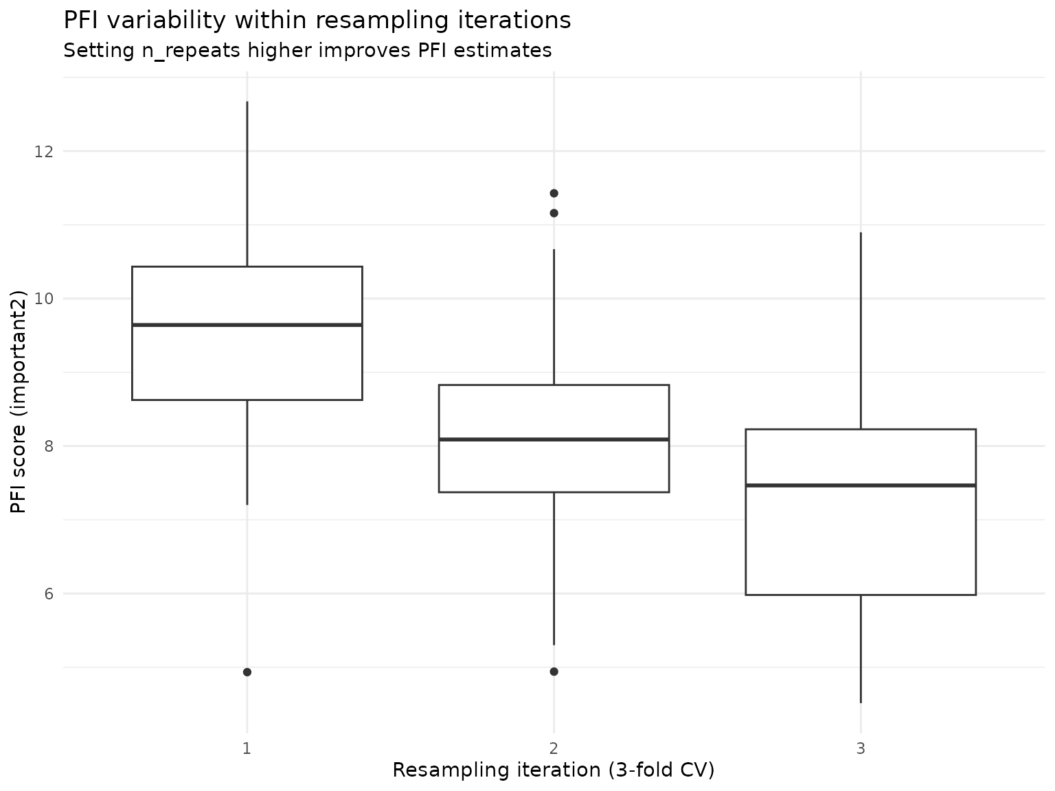
The aggregated importance score for this feature is approximately
8.8, but across all resamplings the estimated PFI scores range from 5.93
to 12.74, and with insufficient resampling or low
n_repeats, we might have over- or underestimated the
features PFI by some margin.
We can also use the ratio of performance scores instead of their difference for the importance calculation, meaning that an unimportant feature is now expected to get an importance score of 1 rather than 0:
pfi_stable$importance(relation = "ratio")
#> Key: <feature>
#>          feature importance
#>           <char>      <num>
#>  1:   important1  2.0243082
#>  2:   important2  2.4624805
#>  3:   important3  1.1991376
#>  4:   important4  3.0667250
#>  5:   important5  1.3191694
#>  6: unimportant1  0.9978850
#>  7: unimportant2  1.0266634
#>  8: unimportant3  1.0061687
#>  9: unimportant4  1.0137466
#> 10: unimportant5  0.9895111
Leave-One-Covariate-Out (LOCO)
LOCO measures importance by retraining the model without each feature and comparing performance to the full model. This shows the contribution of each feature when all other features are present.
loco <- LOCO$new(
    task = task,
    learner = learner,
    measure = measure,
    resampling = resampling,
    n_repeats = 10
)

loco$compute()
loco$importance()
#> Key: <feature>
#>          feature importance
#>           <char>      <num>
#>  1:   important1  3.3430096
#>  2:   important2  4.7465412
#>  3:   important3  0.6079202
#>  4:   important4  7.2998327
#>  5:   important5  0.5541375
#>  6: unimportant1 -0.5955017
#>  7: unimportant2 -0.6082412
#>  8: unimportant3 -0.4519835
#>  9: unimportant4 -0.4972118
#> 10: unimportant5 -0.4346899
LOCO is computationally expensive as it requires retraining for each feature, but provides clear interpretation: higher values mean larger performance drop when the feature is removed. However, it cannot distinguish between direct effects and indirect effects through correlated features.
Feature Samplers
For advanced methods that account for feature dependencies,
xplainfi provides different sampling strategies. While PFI
uses simple permutation (marginal sampling), conditional samplers can
preserve feature relationships.
Let’s demonstrate conditional sampling using adversarial random forests (ARF), which preserves relationships between features when sampling:
arf_sampler <- ConditionalARFSampler$new(task)

sample_data <- task$data(rows = 1:5)
sample_data[, .(important1, important2)]
#>    important1  important2
#>         <num>       <num>
#> 1:  0.2875775 0.784575267
#> 2:  0.7883051 0.009429905
#> 3:  0.4089769 0.779065883
#> 4:  0.8830174 0.729390652
#> 5:  0.9404673 0.630131853
Now we’ll conditionally sample the important1 feature
given the values of important2 and
important3:
sampled_conditional <- arf_sampler$sample_newdata(
    feature = "important1",
    newdata = sample_data,
    conditioning_set = c("important2", "important3")
)

sample_data[, .(important1, important2, important3)]
#>    important1  important2 important3
#>         <num>       <num>      <num>
#> 1:  0.2875775 0.784575267  0.2372297
#> 2:  0.7883051 0.009429905  0.6864904
#> 3:  0.4089769 0.779065883  0.2258184
#> 4:  0.8830174 0.729390652  0.3184946
#> 5:  0.9404673 0.630131853  0.1739838
sampled_conditional[, .(important1, important2, important3)]
#>    important1  important2 important3
#>         <num>       <num>      <num>
#> 1:  0.8502091 0.784575267  0.2372297
#> 2: -0.1656936 0.009429905  0.6864904
#> 3:  0.3339015 0.779065883  0.2258184
#> 4:  0.7164983 0.729390652  0.3184946
#> 5:  0.6126986 0.630131853  0.1739838
This conditional sampling is essential for methods like CFI and RFI
that need to preserve feature dependencies. See the perturbation-importance
article for detailed comparisons and
vignette("feature-samplers") for more details on
implemented samplers.
Detailed Scoring Information
All methods store detailed scoring information from each resampling iteration for further analysis. Let’s examine the structure of PFI’s detailed scores:
pfi$scores() |>
    head(10) |>
knitr::kable(digits = 4, caption = "Detailed PFI scores (first 10 rows)")| feature | iter_rsmp | iter_repeat | regr.mse_baseline | regr.mse_post | importance |
|---|---|---|---|---|---|
| important1 | 1 | 1 | 4.3358 | 8.4459 | 4.1102 |
| important1 | 1 | 2 | 4.3358 | 10.9707 | 6.6349 |
| important1 | 1 | 3 | 4.3358 | 8.6713 | 4.3355 |
| important1 | 1 | 4 | 4.3358 | 8.0078 | 3.6720 |
| important1 | 1 | 5 | 4.3358 | 8.9719 | 4.6362 |
| important1 | 1 | 6 | 4.3358 | 8.9658 | 4.6300 |
| important1 | 1 | 7 | 4.3358 | 9.3660 | 5.0302 |
| important1 | 1 | 8 | 4.3358 | 8.3508 | 4.0150 |
| important1 | 1 | 9 | 4.3358 | 7.9364 | 3.6006 |
| important1 | 1 | 10 | 4.3358 | 9.2786 | 4.9428 |
We can also summarize the scoring structure:
pfi$scores()[, .(
    features = uniqueN(feature),
    resampling_folds = uniqueN(iter_rsmp),
    permutation_iters = uniqueN(iter_repeat),
    total_scores = .N
)]
#>    features resampling_folds permutation_iters total_scores
#>       <int>            <int>             <int>        <int>
#> 1:       10                3                10          300
So $importance() always gives us the aggregated
importances across multiple resampling- and permutation-/refitting
iterations, whereas $scores() gives you the individual
scores as calculated by the supplied measure and the
corresponding importance calculated from the difference of these scores
by default.
Analogous to $importance(), you can also use
relation = "ratio" here:
pfi$scores(relation = "ratio") |>
    head(10) |>
knitr::kable(digits = 4, caption = "PFI scores using the ratio (first 10 rows)")| feature | iter_rsmp | iter_repeat | regr.mse_baseline | regr.mse_post | importance |
|---|---|---|---|---|---|
| important1 | 1 | 1 | 4.3358 | 8.4459 | 1.9480 |
| important1 | 1 | 2 | 4.3358 | 10.9707 | 2.5303 |
| important1 | 1 | 3 | 4.3358 | 8.6713 | 1.9999 |
| important1 | 1 | 4 | 4.3358 | 8.0078 | 1.8469 |
| important1 | 1 | 5 | 4.3358 | 8.9719 | 2.0693 |
| important1 | 1 | 6 | 4.3358 | 8.9658 | 2.0679 |
| important1 | 1 | 7 | 4.3358 | 9.3660 | 2.1602 |
| important1 | 1 | 8 | 4.3358 | 8.3508 | 1.9260 |
| important1 | 1 | 9 | 4.3358 | 7.9364 | 1.8304 |
| important1 | 1 | 10 | 4.3358 | 9.2786 | 2.1400 |
Observation-wise losses and importances
For methods where importances are calculated based on
observation-level comparisons and with decomposable measures, we can
also retrieve observation-level information with
$obs_loss(), which works analogously to
$scores() and $importance() but at an even
more detailed level:
pfi$obs_loss()
#>             feature iter_rsmp iter_repeat row_ids loss_baseline   loss_post
#>              <char>     <int>       <int>   <int>         <num>       <num>
#>     1:   important1         1           1       1     3.3403244  0.26184209
#>     2:   important1         1           1       9     0.4640003  0.00316609
#>     3:   important1         1           1      11     1.0938319 10.11218211
#>     4:   important1         1           1      12     2.0091331  2.28764800
#>     5:   important1         1           1      15    11.4484770 38.11092543
#>    ---
#> 29996: unimportant5         3          10     290    16.8041217 15.25727404
#> 29997: unimportant5         3          10     294     0.4212832  0.31602332
#> 29998: unimportant5         3          10     295     8.0016602  7.86721528
#> 29999: unimportant5         3          10     296     0.2308082  0.18523584
#> 30000: unimportant5         3          10     298    18.8129904 20.48257193
#>        obs_importance
#>                 <num>
#>     1:    -3.07848231
#>     2:    -0.46083425
#>     3:     9.01835017
#>     4:     0.27851489
#>     5:    26.66244838
#>    ---
#> 29996:    -1.54684765
#> 29997:    -0.10525993
#> 29998:    -0.13444495
#> 29999:    -0.04557236
#> 30000:     1.66958152
Since we computed PFI using the mean squared error
(msr("regr.mse")), we can use the associated
Measure$obs_loss(), the squared error.
In the resulting table we see
-
loss_baseline: The loss (squared error) for the baseline model before permutation -
loss_post: The loss for this observation after permutation (or in the case ofLOCO, after refit) -
obs_importance: The difference (or ratio ifrelation = "ratio") of the two losses
Note that not all measures have a Measure$obs_loss():
Some measures like msr("classif.auc") are not decomposable,
so observation-wise loss values are not available.
In other cases, the corresponding obs_loss() is just not
yet implemented in mlr3measures,
but will likely be in the future.
Statistical Inference
All importance methods support confidence intervals and p-values via
the ci_method argument in $importance().
Available approaches range from empirical quantiles and corrected
t-tests (Nadeau & Bengio) for resampling-based variability, to
observation-wise inference methods like CPI/cARFi (for CFI)
and Lei et al. (2018) (for LOCO). Multiplicity correction
via p_adjust is supported for all methods that produce
p-values.
For a comprehensive guide covering all inference methods, see the Inference for Feature Importance article.
Using Pre-trained Learners
By default, xplainfi trains the learner internally via
mlr3::resample(). However, if you have already trained a
learner (for example because training is expensive or you want to
explain a specific model) you can pass it directly to perturbation-based
methods (PFI, CFI, RFI) and
SAGE methods. Refit-based methods (LOCO /
WVIM) require retraining by design and will warn if given a
pretrained learner. The only requirement is that the
resampling must be instantiated and have exactly one
iteration (i.e., a single test set). This is necessary because a
pre-trained learner corresponds to a single fitted model, and there is
no meaningful way to associate it with multiple resampling folds.
A holdout resampling is the natural choice here. We first train the
learner on the train set and PFI will calculate importance
using the trained learner and the corresponding test set defined by the
resampling:
resampling_holdout <- rsmp("holdout")$instantiate(task)
learner_trained <- lrn("regr.ranger", num.trees = 100)
learner_trained$train(task, row_ids = resampling_holdout$train_set(1))

pfi_pretrained <- PFI$new(
    task = task,
    learner = learner_trained,
    measure = measure,
    resampling = resampling_holdout,
    n_repeats = 10
)

pfi_pretrained$compute()
pfi_pretrained$importance()
#> Key: <feature>
#>          feature   importance
#>           <char>        <num>
#>  1:   important1  6.728510965
#>  2:   important2  8.838636697
#>  3:   important3  1.205915997
#>  4:   important4 13.031767131
#>  5:   important5  1.690985717
#>  6: unimportant1 -0.015699992
#>  7: unimportant2 -0.024724978
#>  8: unimportant3  0.004969437
#>  9: unimportant4  0.077583896
#> 10: unimportant5 -0.041979763
A common real-world scenario is that the learner was trained on some
dataset and you want to explain the model on entirely new, unseen data.
In that case, create a task from the new data (via
as_task_regr() for example) and use
rsmp("custom") to designate all rows as the test set. The
resampling here is purely a technicality used for internal consistency,
and the train set is irrelevant since the learner is already trained. A
utility function rsmp_all_test() can be used as a shortcut
to achieve the same goal.
# Simulate: learner was trained elsewhere, we have new data to use
new_data <- tgen("friedman1")$generate(n = 100)

# Same as rsmp_all_test(task)
resampling_custom <- rsmp("custom")$instantiate(
    new_data,
    train_sets = list(integer(0)),
    test_sets = list(new_data$row_ids)
)

pfi_newdata <- PFI$new(
    task = new_data,
    learner = learner_trained,
    measure = measure,
    resampling = resampling_custom,
    n_repeats = 10
)

pfi_newdata$compute()
pfi_newdata$importance()
#> Key: <feature>
#>          feature    importance
#>           <char>         <num>
#>  1:   important1  6.7759279691
#>  2:   important2  8.2868297756
#>  3:   important3  0.6668026485
#>  4:   important4 11.8804933067
#>  5:   important5  1.5529025512
#>  6: unimportant1 -0.0251120766
#>  7: unimportant2  0.0402123498
#>  8: unimportant3  0.0002462674
#>  9: unimportant4  0.0554416808
#> 10: unimportant5 -0.0473285402
If you pass a trained learner with a multi-fold or non-instantiated resampling, you will get an informative error at construction time:
PFI$new(
    task = task,
    learner = learner_trained,
    measure = measure,
    resampling = rsmp("cv", folds = 3)
)
#> Error in `super$initialize()`:
#> ! A pre-trained <Learner> requires an instantiated <Resampling>
#> ℹ Instantiate the <Resampling> before passing it, e.g.
#>   `rsmp("holdout")$instantiate(task)`
Parallelization
Both PFI/CFI/RFI and LOCO/WVIM support parallel execution to speed up
computation when working with multiple features or expensive learners.
The parallelization follows mlr3’s approach, allowing users to choose
between mirai and future backends.
Example with future
The future package provides a simple interface for
parallel and distributed computing:
library(future)
plan("multisession", workers = 2)

# PFI with parallelization across features
pfi_parallel = PFI$new(
    task,
    learner = lrn("regr.ranger"),
    measure = msr("regr.mse"),
    n_repeats = 10
)
pfi_parallel$compute()
pfi_parallel$importance()

# LOCO with parallelization (uses mlr3fselect internally)
loco_parallel = LOCO$new(
    task,
    learner = lrn("regr.ranger"),
    measure = msr("regr.mse")
)
loco_parallel$compute()
loco_parallel$importance()