Inference for Feature Importance

library(xplainfi)
library(mlr3learners)
#> Loading required package: mlr3
library(data.table)
library(ggplot2)

There are multiple inference methods available for different importance methods and estimation targets. The approaches fall into two broad categories:

1. Resampling-based variability: When importance is estimated via resampling (e.g., subsampling), we obtain multiple importance estimates across iterations. We can summarize this variability descriptively (empirical quantiles), or use parametric methods, either naive (raw CIs) or corrected for the dependence structure of resampling (Nadeau & Bengio).

2. Observation-wise inference on test data: When a dedicated test set with i.i.d. observations is available (e.g., holdout), we can use observation-wise loss differences for formal statistical inference. This is the basis for CPI/cARFi (conditional importance) and the Lei et al. method (LOCO inference).

Setup

We use a simple linear DGP for demonstration purposes where

• \(X_1\) and \(X_2\) are strongly correlated (r = 0.7)
• \(X_1\) and \(X_3\) have an effect on Y
• \(X_2\) and \(X_4\) don’t have an effect

task = sim_dgp_correlated(n = 2000, r = 0.7)
learner = lrn("regr.ranger", num.trees = 500)
measure = msr("regr.mse")

DAG for correlated features DGP

Resampling-based variability

When we compute feature importance with resampling — for example, subsampling with multiple repeats — each resampling iteration yields a separate importance estimate. By default, $importance() simply averages these estimates without reporting any measure of variability:

pfi = PFI$new(
    task = task,
    learner = learner,
    resampling = rsmp("subsampling", repeats = 15),
    measure = measure,
    n_repeats = 20 # for stability within resampling iters
)

pfi$compute()
pfi$importance()
#> Key: <feature>
#>    feature   importance
#>     <char>        <num>
#> 1:      x1  6.476555494
#> 2:      x2  0.095842584
#> 3:      x3  1.793989195
#> 4:      x4 -0.000962437

There are several ways to quantify the variability of these estimates, ranging from purely descriptive to parametric inference.

Empirical quantiles

The simplest approach is to look at the empirical distribution of importance scores across resampling iterations. This is not a formal inference method — it merely describes the observed variability without any distributional assumptions.

The "quantile" method returns only confidence bounds (conf_lower, conf_upper) without se, statistic, or p.value, since empirical quantiles are not a statistical test. The conf_* naming is kept for consistency with other methods to ease visualization.

pfi_ci_quantile = pfi$importance(ci_method = "quantile", alternative = "two.sided")
pfi_ci_quantile
#> Key: <feature>
#>    feature   importance   conf_lower   conf_upper
#>     <char>        <num>        <num>        <num>
#> 1:      x1  6.476555494  6.108602488 6.8752121255
#> 2:      x2  0.095842584  0.071144370 0.1213703258
#> 3:      x3  1.793989195  1.736434146 1.8848348302
#> 4:      x4 -0.000962437 -0.003342628 0.0006686405

Raw confidence intervals

A natural next step is to assume the importance scores are approximately normally distributed across resampling iterations and compute t-based confidence intervals. However, these unadjusted confidence intervals are too narrow and hence invalid for inference: the resampling iterations share overlapping training sets, violating the independence assumption underlying the t-distribution.

pfi_ci_raw = pfi$importance(ci_method = "raw", alternative = "two.sided")
pfi_ci_raw
#> Key: <feature>
#>    feature   importance           se  statistic      p.value  conf_lower
#>     <char>        <num>        <num>      <num>        <num>       <num>
#> 1:      x1  6.476555494 0.0707450088  91.547879 7.519530e-21  6.32482254
#> 2:      x2  0.095842584 0.0042155496  22.735490 1.879277e-12  0.08680113
#> 3:      x3  1.793989195 0.0132950768 134.936355 3.311520e-23  1.76547409
#> 4:      x4 -0.000962437 0.0002849623  -3.377418 4.511052e-03 -0.00157362
#>       conf_upper
#>            <num>
#> 1:  6.6282884472
#> 2:  0.1048840389
#> 3:  1.8225042988
#> 4: -0.0003512536

The parametric CI methods ("raw" and "nadeau_bengio") return se, statistic, p.value, conf_lower, and conf_upper. The alternative parameter controls whether a one-sided test ("greater", the default, testing H0: importance <= 0) or two-sided test ("two.sided") is performed. Here we use alternative = "two.sided" for visualization purposes so that conf_upper is finite.

Corrected t-test (Nadeau & Bengio)

To account for the dependence between resampling iterations, we can use the correction proposed by Nadeau & Bengio (2003) and recommended by Molnar et al. (2023). This inflates the variance estimate to account for the overlap between training sets, yielding wider (and more honest) confidence intervals:

pfi_ci_corrected = pfi$importance(ci_method = "nadeau_bengio", alternative = "two.sided")
pfi_ci_corrected
#> Key: <feature>
#>    feature   importance           se statistic      p.value   conf_lower
#>     <char>        <num>        <num>     <num>        <num>        <num>
#> 1:      x1  6.476555494 0.2063236235 31.390276 2.231930e-14  6.034035333
#> 2:      x2  0.095842584 0.0122944003  7.795629 1.848448e-06  0.069473718
#> 3:      x3  1.793989195 0.0387743032 46.267477 1.027030e-16  1.710826586
#> 4:      x4 -0.000962437 0.0008310757 -1.158062 2.662136e-01 -0.002744917
#>      conf_upper
#>           <num>
#> 1: 6.9190756552
#> 2: 0.1222114505
#> 3: 1.8771518043
#> 4: 0.0008200431

The Nadeau-Bengio correction provides better (but still imperfect) coverage compared to the raw approach.

Comparison

To highlight the differences between all three approaches, we visualize them side by side:

pfi_cis = rbindlist(
    list(
        pfi_ci_raw[, type := "raw"],
        pfi_ci_corrected[, type := "nadeau_bengio"],
        pfi_ci_quantile[, type := "quantile"]
    ),
    fill = TRUE
)

ggplot(pfi_cis, aes(y = feature, color = type)) +
    geom_errorbar(
        aes(xmin = conf_lower, xmax = conf_upper),
        position = position_dodge(width = 0.6),
        width = .5
    ) +
    geom_point(aes(x = importance), position = position_dodge(width = 0.6)) +
    scale_color_brewer(palette = "Set2") +
    labs(
        title = "Parametric & non-parametric CI methods",
        subtitle = "RF with 15 subsampling iterations",
        color = NULL
    ) +
    theme_minimal(base_size = 14) +
    theme(legend.position = "bottom")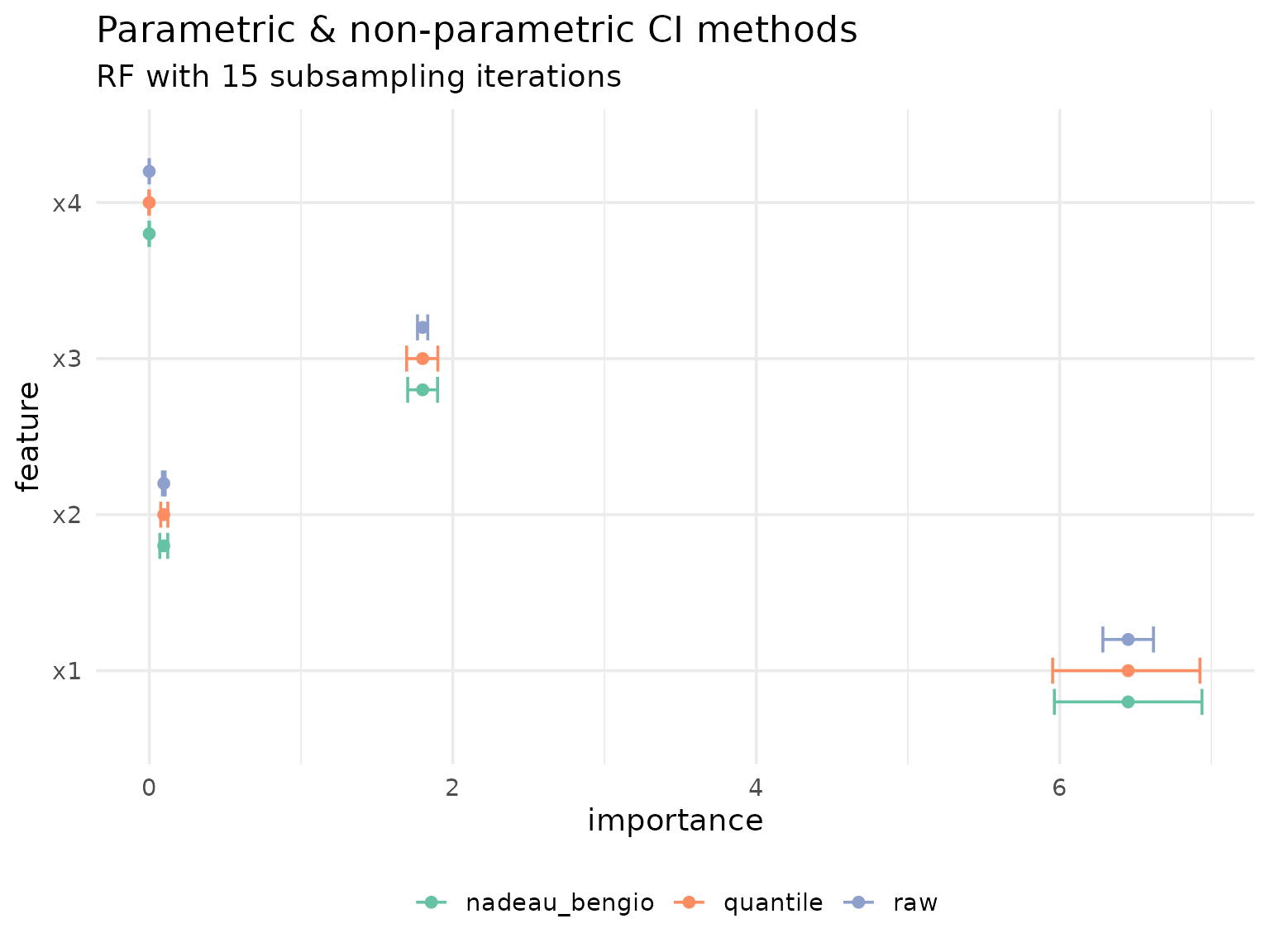

The results highlight just how optimistic the unadjusted, raw confidence intervals are.

Multiplicity correction

When testing many features simultaneously, p-values should be adjusted to control the overall error rate. There are two main frameworks for multiplicity correction:

• Family-wise error rate (FWER): The probability of making at least one false rejection among all tests. FWER control is the more conservative approach and is appropriate when any single false positive would be costly. Methods include Bonferroni (\(\alpha / k\)) and Holm (a step-down variant that is uniformly more powerful than Bonferroni while still controlling FWER).

• False discovery rate (FDR): The expected proportion of false rejections among all rejected hypotheses. FDR control is less conservative and better suited for exploratory analyses where some false positives are tolerable. The most common method is Benjamini-Hochberg (BH).

The p_adjust parameter accepts any method from stats::p.adjust.methods and defaults to "none" (no adjustment).

pfi$importance(ci_method = "nadeau_bengio", alternative = "two.sided", p_adjust = "none")
#> Key: <feature>
#>    feature   importance           se statistic      p.value   conf_lower
#>     <char>        <num>        <num>     <num>        <num>        <num>
#> 1:      x1  6.476555494 0.2063236235 31.390276 2.231930e-14  6.034035333
#> 2:      x2  0.095842584 0.0122944003  7.795629 1.848448e-06  0.069473718
#> 3:      x3  1.793989195 0.0387743032 46.267477 1.027030e-16  1.710826586
#> 4:      x4 -0.000962437 0.0008310757 -1.158062 2.662136e-01 -0.002744917
#>      conf_upper
#>           <num>
#> 1: 6.9190756552
#> 2: 0.1222114505
#> 3: 1.8771518043
#> 4: 0.0008200431

With Bonferroni correction (FWER control), both p-values and confidence intervals are adjusted. The confidence intervals use an adjusted significance level of \(\alpha / k\) where \(k\) is the number of features:

pfi$importance(ci_method = "nadeau_bengio", alternative = "two.sided", p_adjust = "bonferroni")
#> Key: <feature>
#>    feature   importance           se statistic      p.value   conf_lower
#>     <char>        <num>        <num>     <num>        <num>        <num>
#> 1:      x1  6.476555494 0.2063236235 31.390276 8.927721e-14  5.748317045
#> 2:      x2  0.095842584 0.0122944003  7.795629 7.393792e-06  0.052448353
#> 3:      x3  1.793989195 0.0387743032 46.267477 4.108119e-16  1.657131680
#> 4:      x4 -0.000962437 0.0008310757 -1.158062 1.000000e+00 -0.003895796
#>     conf_upper
#>          <num>
#> 1: 7.204793944
#> 2: 0.139236816
#> 3: 1.930846710
#> 4: 0.001970922

For sequential or adaptive procedures such as Holm (FWER) or Benjamini-Hochberg (FDR), only p-values are adjusted. These methods do not yield a clean per-comparison \(\alpha\) that could be used for CI construction, so confidence intervals remain at the nominal level:

pfi$importance(ci_method = "nadeau_bengio", alternative = "two.sided", p_adjust = "BH")
#> Key: <feature>
#>    feature   importance           se statistic      p.value   conf_lower
#>     <char>        <num>        <num>     <num>        <num>        <num>
#> 1:      x1  6.476555494 0.2063236235 31.390276 4.463861e-14  6.034035333
#> 2:      x2  0.095842584 0.0122944003  7.795629 2.464597e-06  0.069473718
#> 3:      x3  1.793989195 0.0387743032 46.267477 4.108119e-16  1.710826586
#> 4:      x4 -0.000962437 0.0008310757 -1.158062 2.662136e-01 -0.002744917
#>      conf_upper
#>           <num>
#> 1: 6.9190756552
#> 2: 0.1222114505
#> 3: 1.8771518043
#> 4: 0.0008200431

This applies to all ci_methods that produce p-values ("raw", "nadeau_bengio", "cpi", "lei").

Observation-wise inference on test data

The resampling-based approaches above quantify variability due to the choice of train/test split. A different approach uses observation-wise loss differences on a test set for formal statistical inference.

The idea is straightforward: for each test observation, we compare the loss with and without a feature (either by perturbing the feature or by retraining the model without it). The resulting per-observation importance scores are i.i.d. under appropriate conditions, enabling standard statistical tests.

Inference is guaranteed to be valid with a single train/test split (holdout), where test observations are truly i.i.d. and the model is fixed. Other resampling strategies may be used but come with caveats (see below).

• CPI / cARFi for conditional feature importance (perturbation-based, model is fixed per resampling iteration)
• Lei et al. for LOCO importance (retraining-based, model is refitted without each feature)

Conditional predictive impact (CPI)

CPI (Conditional Predictive Impact) was introduced by Watson & Wright (2021) for statistical inference with conditional feature importance using knockoffs. Two main approaches are supported:

• CPI with knockoffs: The original method using model-X knockoffs for conditional sampling.
• cARFi (Blesch et al., 2025): Uses Adversarial Random Forests for conditional sampling, which works without Gaussian assumptions and supports mixed data. CPI is originally implemented by the cpi package. It works with mlr3 and its output on our data looks like this:

library(cpi)

resampling = rsmp("cv", folds = 5)
resampling$instantiate(task)

cpi_res = cpi(
    task = task,
    learner = learner,
    resampling = resampling,
    measure = measure,
    test = "t"
)
setDT(cpi_res)
setnames(cpi_res, "Variable", "feature")
cpi_res[, method := "CPI"]

cpi_res
#>    feature           CPI          SE   test  statistic      estimate
#>     <char>         <num>       <num> <char>      <num>         <num>
#> 1:      x1  4.5092929912 0.147978747      t 30.4725717  4.5092929912
#> 2:      x2  0.0029567621 0.003362453      t  0.8793467  0.0029567621
#> 3:      x3  1.8536055915 0.060102228      t 30.8408797  1.8536055915
#> 4:      x4 -0.0008885688 0.000770307      t -1.1535255 -0.0008885688
#>          p.value        ci.lo method
#>            <num>        <num> <char>
#> 1: 3.859678e-168  4.265776760    CPI
#> 2:  1.896595e-01 -0.002576545    CPI
#> 3: 1.768282e-171  1.754700388    CPI
#> 4:  8.755837e-01 -0.002156198    CPI

CPI with knockoffs

Since xplainfi also includes knockoffs via the KnockoffSampler and the KnockoffGaussianSampler, the latter implementing the second order Gaussian knockoffs also used by default in cpi, we can recreate its results using CFI with the corresponding sampler.

CFI with a knockoff sampler supports CPI inference directly via ci_method = "cpi".

knockoff_gaussian = KnockoffGaussianSampler$new(task)

cfi = CFI$new(
    task = task,
    learner = learner,
    resampling = resampling,
    measure = measure,
    sampler = knockoff_gaussian,
    n_repeats = 1 # generate 1 knockoff matrix, like cpi()
)

cfi$compute()

cfi_cpi_res = cfi$importance(ci_method = "cpi")
#> Warning: Observation-wise inference was validated with a single test set.
#> ! Current resampling has 5 iterations.
#> ℹ With cross-validation, models are fit on overlapping training data, which may
#>   affect coverage.
#> ℹ With bootstrap or subsampling, test observations are not i.i.d.
#> ℹ See `vignette("inference", package = "xplainfi")` for details.
cfi_cpi_res
#> Key: <feature>
#>    feature   importance           se  statistic       p.value   conf_lower
#>     <char>        <num>        <num>      <num>         <num>        <num>
#> 1:      x1  4.362355571 0.1355320358 32.1868962 1.697321e-183  4.096556727
#> 2:      x2  0.001742650 0.0029223989  0.5963079  5.510371e-01 -0.003988617
#> 3:      x3  1.769344462 0.0548657780 32.2485988 4.580895e-184  1.661744364
#> 4:      x4 -0.000470146 0.0009370589 -0.5017251  6.159162e-01 -0.002307860
#>     conf_upper
#>          <num>
#> 1: 4.628154415
#> 2: 0.007473916
#> 3: 1.876944560
#> 4: 0.001367568

# Rename columns to match cpi package output for comparison
setnames(cfi_cpi_res, c("importance", "conf_lower"), c("CPI", "ci.lo"))
cfi_cpi_res[, method := "CFI+Knockoffs"]

The results should be very similar to those computed by cpi(), so let’s compare them:

rbindlist(list(cpi_res, cfi_cpi_res), fill = TRUE) |>
    ggplot(aes(y = feature, x = CPI, color = method)) +
    geom_point(position = position_dodge(width = 0.3)) +
    geom_errorbar(
        aes(xmin = CPI, xmax = ci.lo),
        position = position_dodge(width = 0.3),
        width = 0.5
    ) +
    scale_color_brewer(palette = "Dark2") +
    labs(
        title = "CPI and CFI with Knockoff sampler",
        subtitle = "RF with 5-fold CV",
        color = NULL
    ) +
    theme_minimal(base_size = 14) +
    theme(legend.position = "top")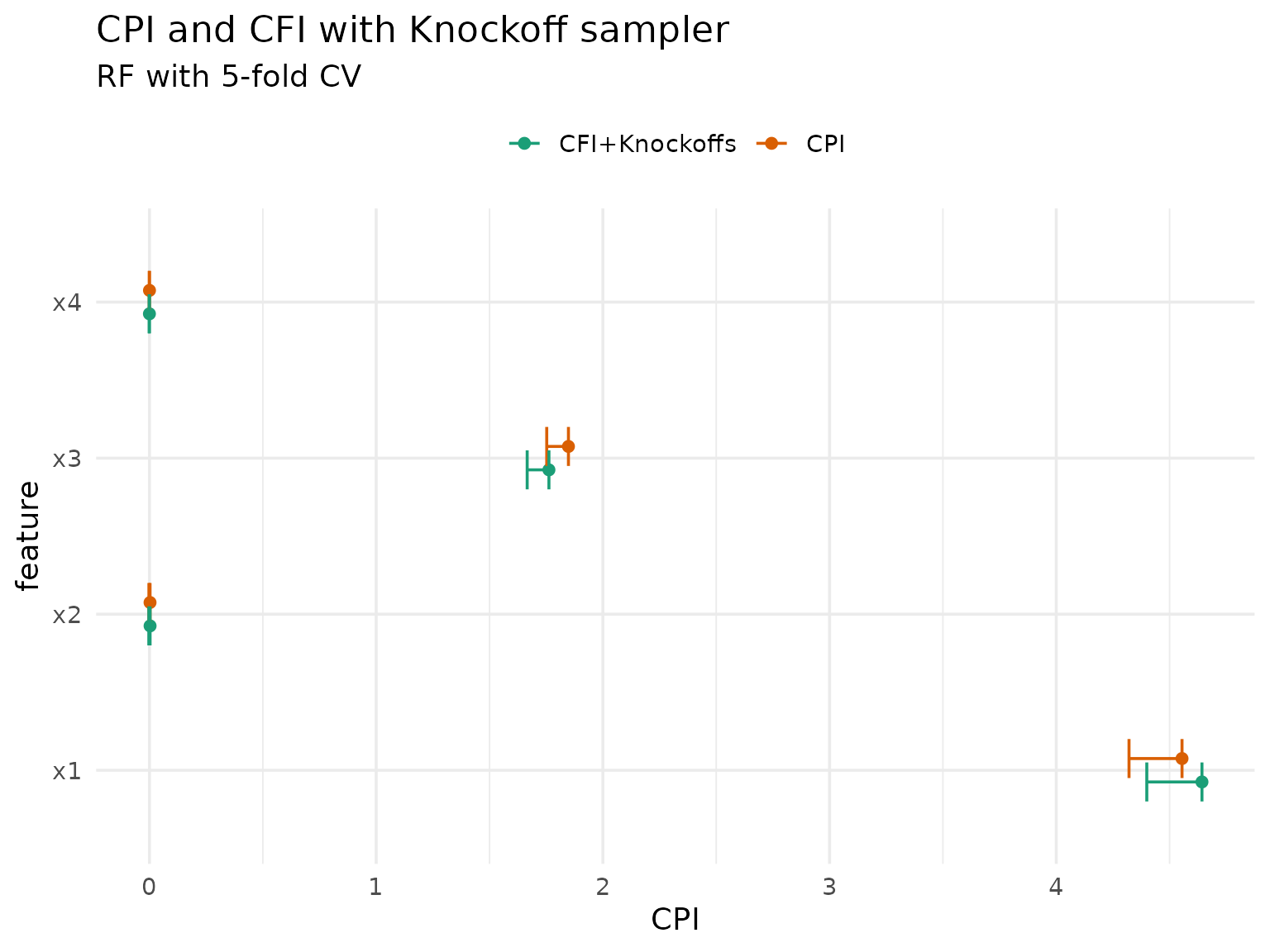

A notable caveat of the knockoff approach is that they are not readily available for mixed data (with categorical features).

cARFi: CPI with ARF

An alternative is available using ARF as conditional sampler rather than knockoffs. This approach, called cARFi, was introduced by Blesch et al. (2025) and works without Gaussian assumptions:

arf_sampler = ConditionalARFSampler$new(
    task = task,
    finite_bounds = "local",
    min_node_size = 20,
    epsilon = 1e-15
)

cfi_arf = CFI$new(
    task = task,
    learner = learner,
    resampling = resampling,
    measure = measure,
    sampler = arf_sampler
)

cfi_arf$compute()

# CPI inference with ARF sampler (cARFi)
cfi_arf_res = cfi_arf$importance(ci_method = "cpi")
#> Warning: Observation-wise inference was validated with a single test set.
#> ! Current resampling has 5 iterations.
#> ℹ With cross-validation, models are fit on overlapping training data, which may
#>   affect coverage.
#> ℹ With bootstrap or subsampling, test observations are not i.i.d.
#> ℹ See `vignette("inference", package = "xplainfi")` for details.
cfi_arf_res
#> Key: <feature>
#>    feature    importance           se statistic    p.value    conf_lower
#>     <char>         <num>        <num>     <num>      <num>         <num>
#> 1:      x1  3.9865071718 0.0715166883 55.742335 0.00000000  3.8462521170
#> 2:      x2  0.0053611218 0.0025570164  2.096632 0.03615158  0.0003464254
#> 3:      x3  1.7527732858 0.0325190020 53.899972 0.00000000  1.6889985989
#> 4:      x4 -0.0009391978 0.0004918991 -1.909330 0.05636256 -0.0019038865
#>      conf_upper
#>           <num>
#> 1: 4.126762e+00
#> 2: 1.037582e-02
#> 3: 1.816548e+00
#> 4: 2.549088e-05

# Rename columns to match cpi package output for comparison
setnames(cfi_arf_res, c("importance", "conf_lower"), c("CPI", "ci.lo"))
cfi_arf_res[, method := "CFI+ARF"]

We can now compare all three methods:

rbindlist(list(cpi_res, cfi_cpi_res, cfi_arf_res), fill = TRUE) |>
    ggplot(aes(y = feature, x = CPI, color = method)) +
    geom_point(position = position_dodge(width = 0.3)) +
    geom_errorbar(
        aes(xmin = CPI, xmax = ci.lo),
        position = position_dodge(width = 0.3),
        width = 0.5
    ) +
    scale_color_brewer(palette = "Dark2") +
    labs(
        title = "CPI and CFI with Knockoffs and ARF",
        subtitle = "RF with 5-fold CV",
        color = NULL
    ) +
    theme_minimal(base_size = 14) +
    theme(legend.position = "top")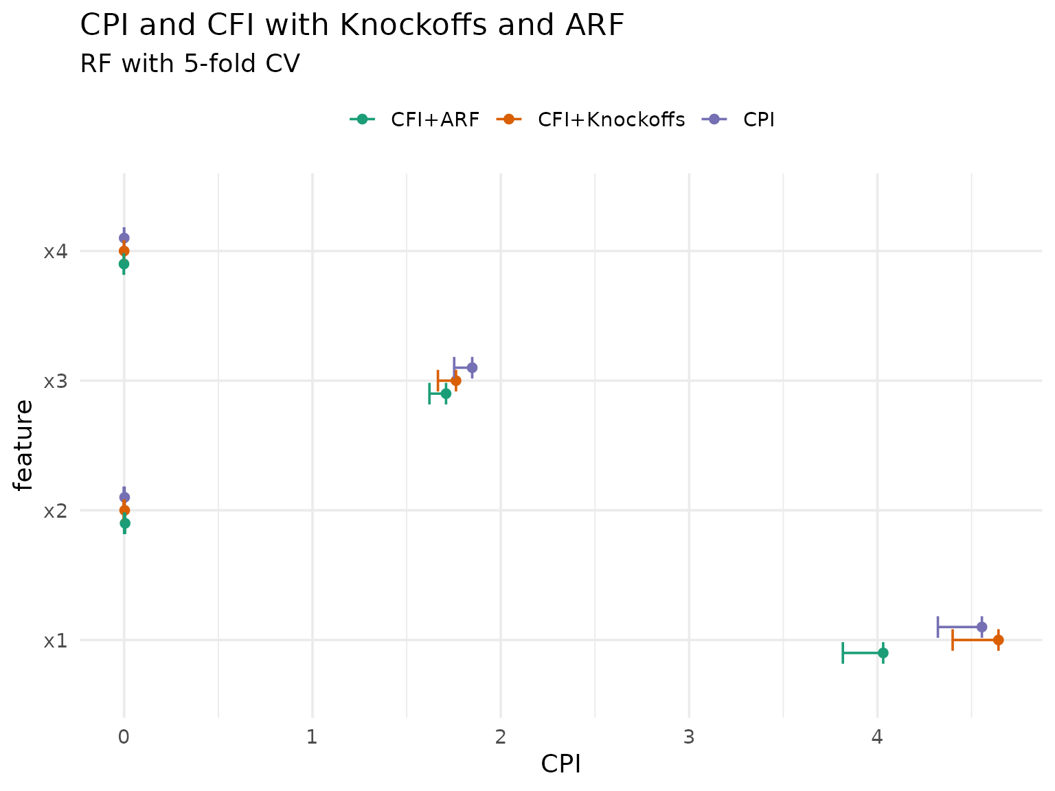

As expected, the ARF-based approach differs more from both knockoff-based approaches, but they are all roughly in agreement.

Note on resampling strategy: CPI inference was validated using holdout (a single train/test split), and inference is provably valid in this setting. With cross-validation, test observations are still i.i.d., but models are fit on overlapping training data — technically, this affects inference for the same reason the Nadeau & Bengio correction exists for resampling-based CIs. With bootstrap or subsampling, test observations may no longer be i.i.d. (due to repeated observations across test sets) and training sets overlap. In practice, Watson & Wright (2021) found that empirical results did not strongly depend on the choice of risk estimator, but inference is only guaranteed to be valid with holdout. Other resampling strategies should be employed with the understanding that coverage guarantees may not hold.

Statistical tests with CPI

CPI can also perform additional tests besides the default t-test, specifically the Wilcoxon-, Fisher-, or binomial test:

(cpi_res_wilcoxon = cfi_arf$importance(ci_method = "cpi", test = "wilcoxon"))
#> Warning: Observation-wise inference was validated with a single test set.
#> ! Current resampling has 5 iterations.
#> ℹ With cross-validation, models are fit on overlapping training data, which may
#>   affect coverage.
#> ℹ With bootstrap or subsampling, test observations are not i.i.d.
#> ℹ See `vignette("inference", package = "xplainfi")` for details.
#> Key: <feature>
#>    feature    importance    se statistic      p.value    conf_lower
#>     <char>         <num> <num>     <num>        <num>         <num>
#> 1:      x1  3.9865071718    NA   2001000 0.000000e+00  3.2122074217
#> 2:      x2  0.0053611218    NA   1194853 5.295553e-14  0.0029276504
#> 3:      x3  1.7527732858    NA   2000886 0.000000e+00  1.3958358130
#> 4:      x4 -0.0009391978    NA   1031351 2.323267e-01 -0.0001657344
#>      conf_upper
#>           <num>
#> 1: 3.4270970290
#> 2: 0.0049551400
#> 3: 1.4966237507
#> 4: 0.0006339549
# Fisher test with same default for B as in cpi()
(cpi_res_fisher = cfi_arf$importance(ci_method = "cpi", test = "fisher", B = 1999))
#> Warning: Observation-wise inference was validated with a single test set.
#> ! Current resampling has 5 iterations.
#> ℹ With cross-validation, models are fit on overlapping training data, which may
#>   affect coverage.
#> ℹ With bootstrap or subsampling, test observations are not i.i.d.
#> ℹ See `vignette("inference", package = "xplainfi")` for details.
#> Key: <feature>
#>    feature    importance    se     statistic p.value    conf_lower   conf_upper
#>     <char>         <num> <num>         <num>   <num>         <num>        <num>
#> 1:      x1  3.9865071718    NA  3.9865071718  0.0005  3.7697941737 4.203211e+00
#> 2:      x2  0.0053611218    NA  0.0053611218  0.0365  0.0001883662 1.032052e-02
#> 3:      x3  1.7527732858    NA  1.7527732858  0.0005  1.6527820910 1.848633e+00
#> 4:      x4 -0.0009391978    NA -0.0009391978  0.0650 -0.0019275157 7.687918e-05
(cpi_res_binom = cfi_arf$importance(ci_method = "cpi", test = "binomial"))
#> Warning: Observation-wise inference was validated with a single test set.
#> ! Current resampling has 5 iterations.
#> ℹ With cross-validation, models are fit on overlapping training data, which may
#>   affect coverage.
#> ℹ With bootstrap or subsampling, test observations are not i.i.d.
#> ℹ See `vignette("inference", package = "xplainfi")` for details.
#> Key: <feature>
#>    feature    importance    se statistic      p.value conf_lower conf_upper
#>     <char>         <num> <num>     <num>        <num>      <num>      <num>
#> 1:      x1  3.9865071718    NA      2000 0.000000e+00  0.9981573  1.0000000
#> 2:      x2  0.0053611218    NA      1215 5.988736e-22  0.5857045  0.6289798
#> 3:      x3  1.7527732858    NA      1995 0.000000e+00  0.9941756  0.9991878
#> 4:      x4 -0.0009391978    NA      1094 2.860106e-05  0.5248785  0.5689835

rbindlist(
    list(
        cfi_arf$importance(ci_method = "cpi")[, test := "t"],
        cpi_res_wilcoxon[, test := "Wilcoxon"],
        cpi_res_fisher[, test := "Fisher"],
        cpi_res_binom[, test := "Binomial"]
    ),
    fill = TRUE
) |>
    ggplot(aes(y = feature, x = importance, color = test)) +
    geom_point(position = position_dodge(width = 0.3)) +
    geom_errorbar(
        aes(xmin = importance, xmax = conf_lower),
        position = position_dodge(width = 0.3),
        width = 0.5
    ) +
    scale_color_brewer(palette = "Dark2") +
    labs(
        title = "CPI test with CFI/ARF",
        subtitle = "RF with 5-fold CV",
        color = "Test"
    ) +
    theme_minimal(base_size = 14) +
    theme(legend.position = "top")
#> Warning: Observation-wise inference was validated with a single test set.
#> ! Current resampling has 5 iterations.
#> ℹ With cross-validation, models are fit on overlapping training data, which may
#>   affect coverage.
#> ℹ With bootstrap or subsampling, test observations are not i.i.d.
#> ℹ See `vignette("inference", package = "xplainfi")` for details.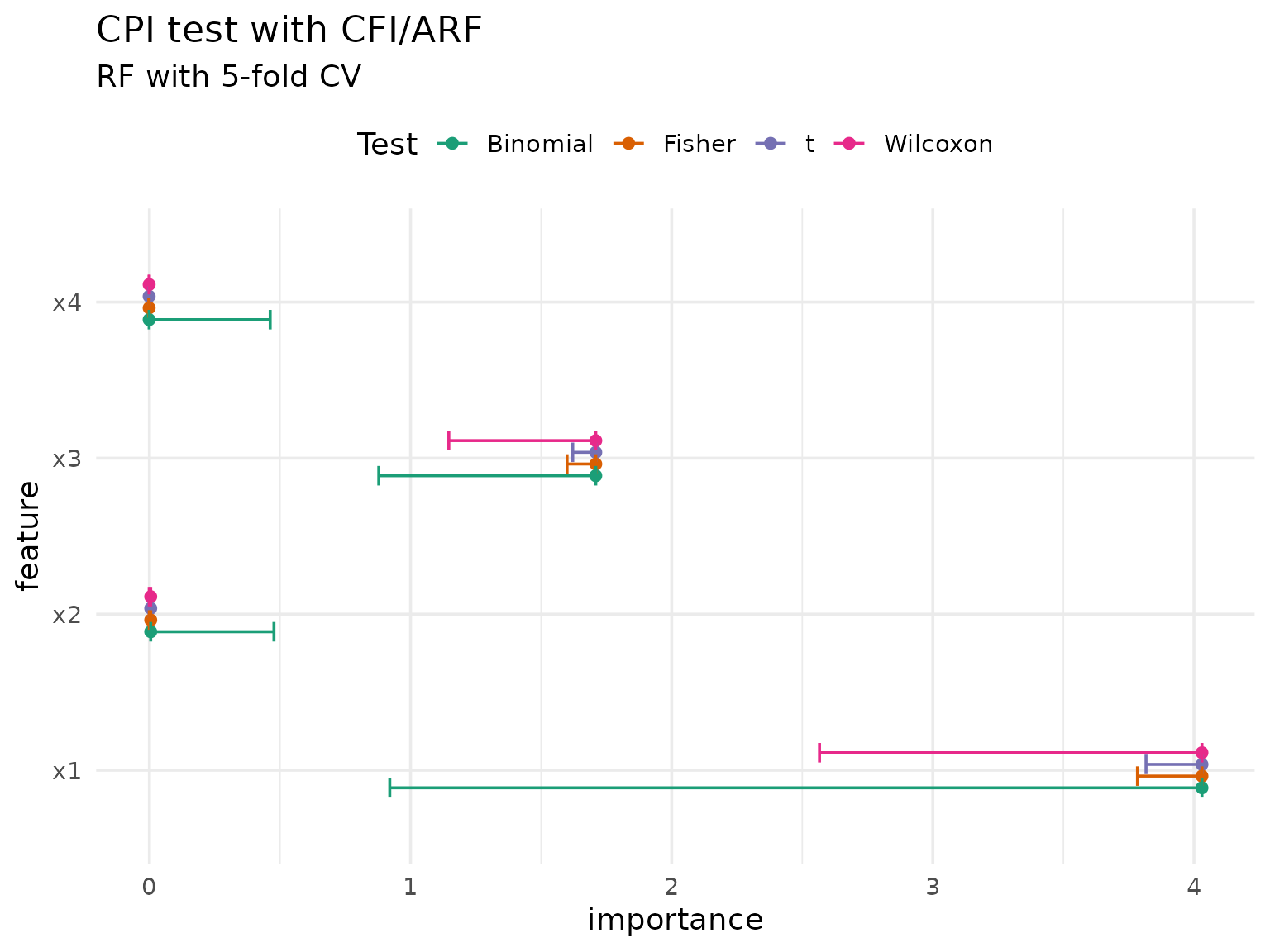

The choice of test depends on distributional assumptions: the t-test assumes normality, while Fisher and Wilcoxon are non-parametric alternatives.

Following Watson & Wright (2021), we can additionally apply Benjamini-Hochberg FDR control (p_adjust = "BH"), which is often desirable in exploratory settings where many features are tested simultaneously:

cfi_arf$importance(ci_method = "cpi", p_adjust = "BH")
#> Warning: Observation-wise inference was validated with a single test set.
#> ! Current resampling has 5 iterations.
#> ℹ With cross-validation, models are fit on overlapping training data, which may
#>   affect coverage.
#> ℹ With bootstrap or subsampling, test observations are not i.i.d.
#> ℹ See `vignette("inference", package = "xplainfi")` for details.
#> Key: <feature>
#>    feature    importance           se statistic    p.value    conf_lower
#>     <char>         <num>        <num>     <num>      <num>         <num>
#> 1:      x1  3.9865071718 0.0715166883 55.742335 0.00000000  3.8462521170
#> 2:      x2  0.0053611218 0.0025570164  2.096632 0.04820210  0.0003464254
#> 3:      x3  1.7527732858 0.0325190020 53.899972 0.00000000  1.6889985989
#> 4:      x4 -0.0009391978 0.0004918991 -1.909330 0.05636256 -0.0019038865
#>      conf_upper
#>           <num>
#> 1: 4.126762e+00
#> 2: 1.037582e-02
#> 3: 1.816548e+00
#> 4: 2.549088e-05

Note that multiplcity adjustment is in the general case limited to p-values, and only the general Bonferroni method is easily applicable to confidence intervals.

Distribution-free inference for LOCO (Lei et al., 2018)

Lei et al. (2018) proposed distribution-free inference for LOCO importance based on observation-wise loss differences. Unlike CPI/cARFi, LOCO requires retraining the model without each feature. The inference is conditional on the training data \(D_1\) from a single train/test split: the observation-wise loss differences on the test set are i.i.d. given \(D_1\), enabling nonparametric tests. The idea is to test whether the excess test error from removing feature \(j\) is significantly greater than zero:

\[ \theta_j = \mathrm{med}\left( |Y - \hat{f}_{n_1}^{-j}(X)| - |Y - \hat{f}_{n_1}(X)| \big| D_1 \right) \]

The paper proposes:

• L1 (absolute) loss as the measure
• Median as the aggregation function
• A single train/test split (holdout), since inference is conditional on the training data
• A Wilcoxon signed-rank test (or sign test) for inference
• Bonferroni correction for multiple comparisons

This is available in xplainfi via ci_method = "lei":

# mae has L1 loss on observation-level, the "mean" aggregation is ignored here
measure_mae = msr("regr.mae")

loco = LOCO$new(
    task = sim_dgp_correlated(n = 2000, r = 0.7),
    learner = lrn("regr.ranger", num.trees = 500),
    resampling = rsmp("holdout"),
    measure = measure_mae
)

loco$compute()
loco$importance(
    ci_method = "lei",
    alternative = "two.sided",
    p_adjust = "bonferroni",
    aggregator = median # default spelled out explicitly
)
#> Key: <feature>
#>    feature importance    se statistic      p.value conf_lower conf_upper
#>     <char>      <num> <num>     <num>        <num>      <num>      <num>
#> 1:      x1 0.80833037    NA    216167 9.828138e-98 0.82052360 1.00057066
#> 2:      x2 0.01819719    NA    135421 5.538819e-06 0.01210851 0.03837064
#> 3:      x3 0.52495928    NA    211296 5.603680e-89 0.51589328 0.64318191
#> 4:      x4 0.01989962    NA    146280 9.639960e-12 0.01774627 0.03932460

The ci_method = "lei" method works on observation-wise loss differences internally, using the median as the default point estimate and the Wilcoxon signed-rank test for confidence intervals and p-values.

Configurable parameters

All components proposed by Lei et al. are the defaults but can be customized:

• test: "wilcoxon" (default), "t", "fisher", or "binomial" (sign test)
• aggregator: defaults to stats::median, can be changed (e.g. mean)
• p_adjust: p-value correction for multiple comparisons, accepts any method from stats::p.adjust.methods (e.g. "bonferroni", "holm", "BH", "none"). Default is "none". When "bonferroni", confidence intervals are also adjusted (alpha/k). For other methods like "holm" or "BH", only p-values are adjusted because these sequential/adaptive procedures do not yield a clean per-comparison alpha for CI construction.

loco$importance(
    ci_method = "lei",
    test = "t",
    aggregator = mean,
    alternative = "two.sided",
    p_adjust = "holm"
)
#> Key: <feature>
#>    feature importance          se statistic       p.value conf_lower conf_upper
#>     <char>      <num>       <num>     <num>         <num>      <num>      <num>
#> 1:      x1 0.97220860 0.033777130 28.783043 2.152723e-118 0.90588611 1.03853109
#> 2:      x2 0.04079587 0.007403802  5.510125  5.128595e-08 0.02625827 0.05533348
#> 3:      x3 0.61203461 0.022878509 26.751508 3.754000e-107 0.56711192 0.65695730
#> 4:      x4 0.04338934 0.005255062  8.256675  1.611160e-15 0.03307085 0.05370782