Training Efficiency

Methods for increasing training efficiency can be roughly split into:

1. Computational methods such as JIT compilation, using GPUs, parallel data loading, etc., that allow doing the same thing faster.
2. Methodological approaches that change how we approach modeling to achieve either better results or the same results faster.

Computational Approaches

Parallel Processing

Graphical Processing Unit (GPU)

Using a GPU is crucial when training relatively large neural networks because GPUs are specifically designed to handle the parallel processing required for complex computations. To use a GPU in mlr3torch, we can set the device parameter to “cuda”. By default, it is set to “auto”, which will use a GPU if available and otherwise fall back to the CPU.

Tip

To check if a GPU is available, we can use the torch::cuda_is_available() function.

library(torch)
cuda_is_available()

[1] FALSE

If you have an M1 Mac (or later), you can also use the available graphics card by setting the device parameter to "mps". You can check this by running:

backends_mps_is_available()

[1] TRUE

To demonstrate the speed improvements obtained by using a GPU, we conduct a large matrix operation on a GPU and a CPU. We start by randomly sampling a matrix of size 1000x1000.

x_cpu = torch_randn(1000, 1000, device = "cpu")

Below, we perform a matrix multiplication on the CPU and the GPU and compare the timings.

# this will only run if a GPU is available
x_cuda = x_cpu$cuda()

bench::mark(
  cpu = x_cpu$matmul(x_cpu),
  cuda = x_cuda$matmul(x_cuda)
)

CPU Threads

Training large networks on a CPU is not a recommended approach, but it can be a viable option for smaller networks. You can still use multiple threads to speed up the execution of operations. Please be aware that the code below will not execute on macOS, as setting the number of threads is not supported on this operating system.

# this will be skipped on macOS
bench::mark(
  {torch_set_num_threads(1L); x_cpu$matmul(x_cpu)},
  {torch_set_num_threads(16L); x_cpu$matmul(x_cpu)}
)

torch also allows for interop-parallelization, but this is more advanced and code needs to be written in a specific way.

Quiz: Number of Threads

Question 1: On a CPU with 4 cores, does it make sense to set the number of threads to values greater than 4? Explain your answer.

Click for answer

On a CPU with 4 cores, at most 4 threads can run in parallel. Using more threads than the number of cores will not speed up the execution of operations.

Question 2: On a CPU with 64 cores, is it always the case that using 64 threads is better than using 32 threads?

Click for answer

Not necessarily. Using more threads will mean that:

1. The threads need to communicate and synchronize, which increases the runtime.
2. More resources are used for the computation, which decreases the runtime.

The optimal number of threads is a trade-off between these two effects.

Efficient Data Loading

Besides parallelizing the computation of operations in the forward and backward pass, another possible bottleneck is the loading of data. There are various ways to improve data loading speed:

1. Improve the implementation of the dataset class
2. Parallelize the data loading process
3. Increase the speed of data transfer to the GPU

These approaches will now be discussed.

Efficient Dataset Implementation

When implementing a dataset, we need to define:

1. How we store and load the data
2. Whether implementing loading of a batch is beneficial

Quiz: Data Loading

The tiny imagenet dataset is a dataset of 100,000 images of size 64x64. It is a subset of the famous imagenet dataset. Below, we show some examples from it:

We will now consider different ways to write a torch::dataset implementation for this data. Assume we have some image paths stored in a character vector as well as in an array where they are already loaded into memory.

str(image_paths)

 chr [1:100] "/Users/sebi/Library/Caches/org.R-project.R/R/mlr3torch/datasets/tiny_imagenet/raw/tiny-imagenet-200/train/n0144"| __truncated__ ...

str(image_array)

 num [1:100, 1:3, 1:64, 1:64] 1 0.0784 0.4706 0.5608 0.5647 ...

An individual image can, for example, be loaded using the torchvision::base_loader() function:

library(torchvision)
str(base_loader(image_paths[1]))

 num [1:64, 1:64, 1:3] 1 1 1 1 1 ...

Question 1: Reading From Disk or RAM

Which of the following is the faster way to load the images? Explain why.

1. Loading the images from disk:

   ds_disk = dataset("image_paths",
     initialize = function(image_paths) {
       self$image_paths = image_paths
     },
     .getitem = function(i) {
       torch_tensor(torchvision::base_loader(self$image_paths[i]))
     },
     .length = function() {
       length(self$image_paths)
     }
   )(image_paths)

2. Loading the images from an array:

   ds_ram = dataset("image_array",
     initialize = function(image_array) {
       self$image_array = image_array
     },
     .getitem = function(i) {
       torch_tensor(self$image_array[i, , , ])
     },
     .length = function() {
       nrow(self$image_array)
     }
   )(image_array)

Click for answer

Generally, loading images from RAM is significantly faster than loading them from disk. Although the benchmark presented below may seem somewhat ‘unfair’ since ds_ram has already loaded the images into memory, this difference is evident in practice. When iterating over the dataset for multiple epochs, the first method will need to reload the images from disk for each epoch, while the second method only requires a single loading of the images into memory.

iter = function(ds, ..., epochs = 1) {
  dl = torch::dataloader(ds, batch_size = 16, ...)
  for (epoch in seq_len(epochs)) {
    coro::loop(for(batch in dl) {
      batch
    })
  }
}
bench::mark(
  disk = iter(ds_disk, epochs = 10),
  ram = iter(ds_ram, epochs = 10),
  check = FALSE
)

Warning: Some expressions had a GC in every iteration; so filtering is disabled.

# A tibble: 2 × 6
  expression      min   median `itr/sec` mem_alloc `gc/sec`
  <bch:expr> <bch:tm> <bch:tm>     <dbl> <bch:byt>    <dbl>
1 disk          228ms    258ms      3.88     109MB     9.69
2 ram           183ms    184ms      5.33    94.4MB    10.7 

Question 2: (Don’t) Copy that

Consider now the next dataset implementation:

ds_tensor = dataset("tensor",
  initialize = function(image_array) {
    self$tensor = torch_tensor(image_array)
  },
  .getitem = function(i) {
    self$tensor[i, ..]
  },
  .length = function() {
    nrow(self$tensor)
  }
)(image_array)

Do you think this implementation is faster or slower than the ds_ram implementation? Explain why.

Click for answer

This implementation is faster than the ds_ram implementation. This is because the ds_tensor implementation copies the R array to a torch tensor only once, whereas the ds_ram implementation copies the R array to a torch tensor for each item.

bench::mark(
  tensor = iter(ds_tensor),
  array = iter(ds_ram),
  check = FALSE
)

# A tibble: 2 × 6
  expression      min   median `itr/sec` mem_alloc `gc/sec`
  <bch:expr> <bch:tm> <bch:tm>     <dbl> <bch:byt>    <dbl>
1 tensor       4.52ms   4.82ms     206.    96.08KB     6.71
2 array       14.94ms  16.26ms      62.0    9.44MB    16.9 

Question 3: $.getbatch() vs $.getitem()

Which implementation is faster? Explain why.

ds_tensor_batch = dataset("tensor_batch",
  initialize = function(image_array) {
    self$tensor = torch_tensor(image_array)
  },
  .getbatch = function(i) {
    self$tensor[i, .., drop = FALSE]
  },
  .length = function() {
    nrow(self$tensor)
  }
)(image_array)

Click for answer

The $.getbatch() implementation is faster than the $.getitem() implementation. This is because when using the $.getitem() method, the batch for indices ids is obtained by calling $.getitem(id) for each index in ids and then stacking them together, which requires a new tensor allocation. Slicing the tensor, however, avoids this allocation when shuffle = TRUE (which is also the default).

bench::mark(
  getbatch = iter(ds_tensor_batch),
  getitem = iter(ds_tensor),
  check = FALSE
)

# A tibble: 2 × 6
  expression      min   median `itr/sec` mem_alloc `gc/sec`
  <bch:expr> <bch:tm> <bch:tm>     <dbl> <bch:byt>    <dbl>
1 getbatch     1.75ms   1.94ms      502.      23KB     4.69
2 getitem      4.61ms   4.94ms      198.    54.7KB     7.54

Parallel Data Loading

In Deep Learning, datasets can be very large, and it might therefore be the case that the data is simply too large to fit into memory. In this case, we can use parallel data loading to speed up the data loading process. Instead of loading the data sequentially in the main process, other R processes will be started that execute the data loading. For example, if we set num_workers = 4L, 4 R processes will be started that load the data, while the main process is free to train the model. These processes then send the batches to the main process. The image below visualizes this process:

Creating such a parallel dataloader is as easy as setting the num_workers parameter to a value greater than 0.

Note

Note that in the current implementation, parallel data loading is only beneficial when it is slow, e.g., because of loading the data from disk or because of expensive preprocessing. This will hopefully be improved in the future (by a faster implementation of the parallel dataloader).

Moving Data to the GPU

One thing we have ignored so far is that when training using a GPU, the data needs to be moved from RAM to the GPU. This is because a GPU has its own memory (VRAM), and the data needs to be moved to this memory before it can be used for training. The moving of the data to the GPU cannot be done on the processes that are loading the data but must be done in the main process, i.e., after the batch was received from (possibly parallelized) dataloader. One way to speed up the data loading process is to pin the memory of the data to the GPU. Before a tensor can be moved from RAM to VRAM, it needs to be in so-called page-locked memory, which can be enabled using the pin_memory parameter of dataloader()..

iter_cuda = function(ds, pin_memory = TRUE) {
  dl = torch::dataloader(ds, batch_size = 16, pin_memory = pin_memory)
  coro::loop(for(batch in dl) {
    batch$cuda()
  })
}

bench::mark(
  not_pinned = iter_cuda(ds_disk, pin_memory = FALSE),
  pinned = iter_cuda(ds_disk, pin_memory = TRUE)
)

Note

In order to use parallel data loading or memory pinning with mlr3torch, these parameters can simply be specified in the learner:

lrn("classif.mlp", num_workers = 8L, pin_memory = TRUE, device = "cuda")

JIT Compilation & Ignite Optimizers

Some special care needs to be taken when using torch (or mlr3torch) in order to get good performance. In the future, this will hopefully not be necessary anymore, but is currently required.

‘Ignite’ Optimizers

In torch, different versions of optimizers exist:

optim_adamw

<optim_adamw> object generator
  Inherits from: <inherit>
  Public:
    initialize: function (params, lr = 0.001, betas = c(0.9, 0.999), eps = 1e-08, 
    loop_fun: function (group, param, g, p) 
    step: function (closure = NULL) 
    clone: function (deep = FALSE) 
  Parent env: <environment: 0x12cfbcbc8>
  Locked objects: FALSE
  Locked class: FALSE
  Portable: TRUE

optim_ignite_adamw

<optim_ignite_adamw> object generator
<optim_ignite> object generator
  Inherits from: <inherit>
  Public:
    initialize: function (params, lr = 0.001, betas = c(0.9, 0.999), eps = 1e-08, 
    clone: function (deep = FALSE) 
  Private:
    .config_names: lr betas eps weight_decay amsgrad
    .state_names: exp_avg exp_avg_sq max_exp_avg_sq step
    .optim: function (params, ...) 
    .get_states: function (opt) 
    .set_states: function (opt, params, states) 
    .add_param_group: function (opt, params, lr, betas, eps, weight_decay, amsgrad) 
    .assert_params: function (lr, betas, eps, weight_decay, amsgrad) 
    .set_param_group_options: function (opt, list) 
    .zero_grad: function (opt) 
    .get_param_groups: function (ptr) 
  Parent env: <environment: 0x12cae2478>
  Locked objects: FALSE
  Locked class: FALSE
  Portable: TRUE

The ‘ignite’ indicates that the optimizer is a version that is optimized for performance. Not for all optimizers does an ignite version exist, but for the most common ones, there does.

Below, we compare the performance of the default optimizer and the ignite optimizer and see that the latter is considerably faster.

adamw = as_torch_optimizer(torch::optim_adamw)
ignite_adamw = as_torch_optimizer(torch::optim_ignite_adamw)

learner = lrn("classif.mlp", epochs = 10, neurons = c(100, 100), batch_size = 32, optimizer = adamw)

learner_ignite = learner$clone(deep = TRUE)
learner_ignite$configure(
  optimizer = ignite_adamw
)
task_sonar = tsk("sonar")

bench::mark(
  learner$train(task_sonar),
  learner_ignite$train(task_sonar),
  check = FALSE
)

Warning: Some expressions had a GC in every iteration; so filtering is disabled.

# A tibble: 2 × 6
  expression                            min   median `itr/sec` mem_alloc `gc/sec`
  <bch:expr>                       <bch:tm> <bch:tm>     <dbl> <bch:byt>    <dbl>
1 learner$train(task_sonar)           588ms    588ms      1.70    15.7MB     5.10
2 learner_ignite$train(task_sonar)    204ms    208ms      4.77    10.7MB     4.77

JIT Compilation

JIT (Just-In-Time) compilation is a runtime optimization technique that compiles code into machine code during execution rather than beforehand. This has different advantages:

1. By JIT-compiling a model, some operations can be optimized for performance.
2. A JIT-compiled model can be saved and executed without an R dependency for deployment (only LibTorch is required), e.g., in a C++ application.
3. Running a JIT-compiled model in R is faster because the whole network is executed in C++ instead of R.

In torch, this can either be done using TorchScript or by tracing a model. We will briefly discuss both approaches, but for more information, see the torch documentation.

TorchScript

TorchScript is a subset of Python – i.e., its own programming language – that can be used to define compiled functions. In R, this is available via the jit_compile function.

f = jit_compile("
def f(x, w, bias):
  return x @ w + bias
")$f

x = torch_randn(10, 10)
w = torch_randn(10, 1)
bias = torch_randn(1)

out = f(x, w, bias)
str(out)

Float [1:10, 1:1]

Besides syntax, there are some notable differences between TorchScript and R to be aware of:

1. In TorchScript, indexing tensors is 0-based, and
2. TorchScript is statically typed, so you need to specify the types of the arguments, unless they are tensors, which is the default.

Below, we define a function that takes a list of tensors and calculates their sum.

sum_jit = jit_compile("
def sum_jit(xs: List[Tensor]):
  output = torch.zeros_like(xs[0])
  for x in xs:
    output = output + x
  return output
")$sum_jit

sum_jit(list(torch_randn(1), torch_randn(1)))

torch_tensor
-0.7121
[ CPUFloatType{1} ]

Tracing

The alternative to writing TorchScript is to write your module in R and to use jit_trace to compile it.

f2 = function(x, w, bias) {
  x$matmul(w) + bias
}
# need to provide some example input
# arguments are passed by position
f2 = jit_trace(f2, torch_randn(10, 10), torch_randn(10, 100), torch_randn(100))
out2 = f2(x, w, bias)
torch_equal(out, out2)

[1] TRUE

An advantage of trace-compilation is that it can be applied to modules, which is currently not possible with jit_compile.

net = nn_sequential(
  nn_linear(10, 100),
  nn_relu(),
  nn_linear(100, 10)
)
net_jit = jit_trace(net, torch_randn(10, 10))

torch_equal(net(x), net_jit(x))

[1] TRUE

However, trace-compilation is restrictive because it only records operations applied to torch tensors and is unaware of R control flow, so you need to be careful when using it. Furthermore, it only accepts torch tensors as arguments. For many simple modules, trace-compilation should usually work. You can also check this by running the original and trace-jitted module on some example inputs and see if they return the same result.

Note

A trace-jitted module does respect the mode of the network, i.e., whether it is training or evaluating.

In mlr3torch, trace compilation is also available and can be enabled by setting jit_trace = TRUE in the learner.

learner = lrn("classif.mlp", jit_trace = TRUE)

You can also combine TorchScript with tracing:

net_both = nn_module(
  initialize = function() {
    self$linear = nn_linear(1, 1)
  },
  forward = function(x) {
    self$linear(sum_jit(x))
  }
)()

net_both(list(torch_randn(1), torch_randn(1)))

torch_tensor
 1.0027
[ CPUFloatType{1} ][ grad_fn = <ViewBackward0> ]

net_both(list(torch_randn(1)))

torch_tensor
0.01 *
 8.5286
[ CPUFloatType{1} ][ grad_fn = <ViewBackward0> ]

Quiz: Just In Time

Question 1: Consider the trace-jitted function below. Can you predict the output of the last two lines? Can you explain why this happens?

f = function(a, b, multiply) {
  if (multiply$item()) {
    a * b
  } else {
    a + b
  }
}
fjit = jit_trace(f, torch_tensor(1), torch_tensor(2), torch_tensor(TRUE))

fjit(torch_tensor(2), torch_tensor(3), torch_tensor(TRUE))
fjit(torch_tensor(2), torch_tensor(3), torch_tensor(FALSE))

Click for answer

fjit(torch_tensor(2), torch_tensor(3), torch_tensor(TRUE))

torch_tensor
 6
[ CPUFloatType{1} ]

fjit(torch_tensor(2), torch_tensor(3), torch_tensor(FALSE))

torch_tensor
 6
[ CPUFloatType{1} ]

Question 2: Answer the same question for the following function:

f = function(a, b, multiply) {
  torch_where(multiply, a * b, a + b)
}
fjit = jit_trace(f, torch_tensor(1), torch_tensor(2), torch_tensor(TRUE))

fjit(torch_tensor(2), torch_tensor(3), torch_tensor(TRUE))
fjit(torch_tensor(2), torch_tensor(3), torch_tensor(FALSE))

Click for answer

fjit(torch_tensor(2), torch_tensor(3), torch_tensor(TRUE))

torch_tensor
 6
[ CPUFloatType{1} ]

fjit(torch_tensor(2), torch_tensor(3), torch_tensor(FALSE))

torch_tensor
 5
[ CPUFloatType{1} ]

Mixed Precision Training

Another way to speed up the training process is to use mixed precision training. This technique involves training the model using both 16-bit and 32-bit floating point numbers. This allows reducing the memory footprint of the model and speeding up the training process. We won’t cover this here, but refer to the torch documentation that explains how to do this.

Methodological Approaches

Validation and Early Stopping

For more details on this topic, see the corresponding chapter in the mlr3 book.

As we have already seen in one of the previous notebooks, in deep learning, some part of the data is often used for validation purposes. This allows monitoring the performance of the model on unseen data.

In mlr3torch, we can track the performance of the model on a validation set by specifying:

• validate, which is the ratio of the data that is used for validation
• measures_valid, which is a list of measures to evaluate the validation performance
• eval_freq, which is the frequency at which the validation is performed
• callbacks, which is a list of callbacks to use during training, in this case, we use the t_clbk("history") callback, which records the performance of the model on the validation set at regular intervals, enabling us to monitor and analyze the model’s performance over time.

task = tsk("sonar")

mlp_learner = lrn("classif.mlp",
  neurons = c(50, 50), batch_size = 256, epochs = 400,
  optimizer = t_opt("adam", lr = 0.003),
  predict_type = "prob", jit_trace = TRUE,
  # Validation / Performance Monitoring
  validate = 0.3, # how much data to use for validation
  measures_valid = msr("classif.logloss"), # how to evaluate train performance
  measures_train = msr("classif.logloss"), # how to evaluate validation performance
  callbacks = t_clbk("history"), # history callbacks save train and validation performance
  eval_freq = 10 # after how many training epochs to perform validation
)
mlp_learner$train(task)
history = mlp_learner$model$callbacks$history
head(history)

Key: <epoch>
   epoch train.classif.logloss valid.classif.logloss
   <num>                 <num>                 <num>
1:    10             0.6775741             0.6665855
2:    20             0.6430574             0.6176948
3:    30             0.5685190             0.5364953
4:    40             0.5151559             0.4694589
5:    50             0.4780497             0.4363074
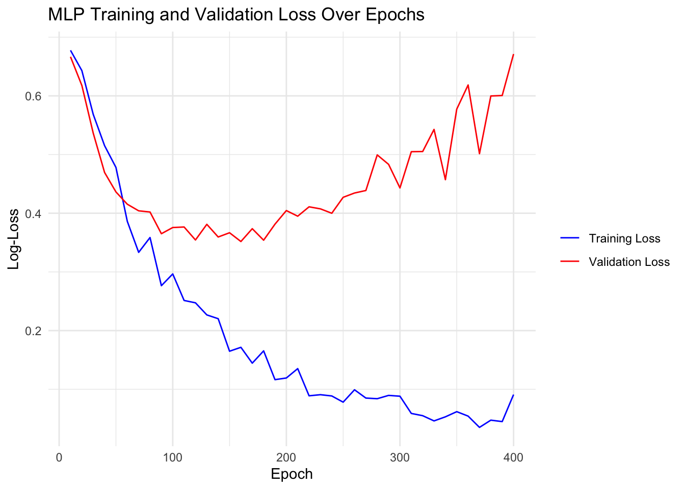
6:    60             0.3861667             0.4153698

Below we plot the training and validation for the different epochs:

Instead of only monitoring the validation loss (and watching it get worse and worse), we can also stop the training process dynamically when the validation loss begins to increase. This regularization technique is called early stopping, and it prevents overfitting during the training of iteratively trained machine learning models.

The key configuration option for early stopping is the patience parameter, which defines the number of epochs to wait after the last improvement in validation loss before stopping the training. For example, if the patience is set to 5, the training will continue for 5 additional epochs after the last observed improvement in validation loss. If no improvement is seen during this period, training will be halted.

Advantages of early stopping include:

• Prevention of Overfitting: By stopping training when the model starts to overfit, we can achieve better generalization on unseen data.
• Resource Efficiency: It saves computational resources by avoiding unnecessary training epochs once the model performance has plateaued.

Now, let’s train the learner again using early stopping with a patience of 5 epochs:

mlp_learner$param_set$set_values(
  patience = 5
)
mlp_learner$train(task)
mlp_learner$internal_tuned_values$epochs

[1] 160

Beyond only tuning the number of epochs, mlr3’s internal tuning mechanism also allows tuning the number of epochs internally while using an offline tuning method to optimize other hyperparameters. To use this, we can set the parameters we want to tune using to_tune(), but need to set internal = TRUE for the epochs parameter.

library(mlr3tuning)
mlp_learner$param_set$set_values(
  epochs = to_tune(upper = 100, internal = TRUE),
  opt.lr = to_tune(lower = 1e-4, upper = 1e-1, logscale = TRUE)
)

We could now pass this learner to a tuner as usual.

Architecture Design

Another essential aspect of training neural networks efficiently and effectively is the design of the network architecture, which can be a challenging task. However, for many problems, there are predefined architectures that perform well and can be used. Unless there is a specific reason to design a new architecture, it is recommended to use such an architecture.

Note

Because the Python deep learning ecosystem is so large, many more architectures are implemented in Python than in R. One way to use them in R is to simply translate the PyTorch code to (R-)torch. While PyTorch and (R-)torch are quite similar, there are some differences, e.g., 1-based and 0-based indexing. The torch website contains a brief tutorial on this topic.

Nonetheless, we will cover important techniques that can be used to speed up the training process, namely batch normalization and dropout.

Batch Normalization

Batch Normalization is an important technique in deep learning that contributed significantly to speeding up the training process.

The formula for batch normalization (during training) is given by:

\[ \hat{x} = \frac{x - \mu_B}{\sqrt{\sigma_B^2 + \epsilon}} \]

where:

• \(\hat{x}\) is the normalized output,
• \(x\) is the input,
• \(\mu_B\) is the mean of the batch,
• \(\sigma_B^2\) is the variance of the batch,
• \(\epsilon\) is a small constant added for numerical stability.

During inference, the module uses the running mean and variance of the training data to normalize the input.

In torch, different versions of batch normalization exist for different dimensions of the input tensor. Below, we illustrate the batch normalization module using a 1D input tensor (the batch dimension does not count here):

x = torch_randn(10, 5)
bn = nn_batch_norm1d(num_features = 5)
bn(x)

torch_tensor
 1.4613 -1.3934 -0.2146  1.0406  0.1413
-0.9634 -0.3388  1.7441  0.7744  2.1476
-2.0328  0.5667 -2.0592  0.4071 -0.0529
 0.6778  0.3264  0.2637 -0.2301 -0.0409
-0.9243  0.1298 -0.6447 -1.5477 -2.1935
 0.8150 -0.1962  0.7988 -1.5426  0.1137
-0.2350 -2.0121 -0.1847  1.1725  0.0143
 0.8381  0.6141  0.9971  1.0148 -0.5667
 0.2166  0.7147 -0.7208 -0.1408 -0.0285
 0.1467  1.5887  0.0203 -0.9482  0.4657
[ CPUFloatType{10,5} ][ grad_fn = <NativeBatchNormBackward0> ]

Quiz: Batch Normalization

Question 1: Earlier we have learned that nn_modules have buffers and parameters, where only the latter are learned with gradient descent. Do you think the mean and variance are parameters or buffers?

Click for answer

They are both buffers as they only store the variance and running mean of all training samples seen, i.e., they are not updated using gradient information.

Question 2: Training vs. Evaluation Mode: While many nn_modules behave the same way irrespective of their mode, batch normalization is an example of a module that behaves differently during training and evaluation. During training, the module uses the mean and variance of the current batch, while during evaluation, it uses the running mean and variance of all training samples seen.

bn(x[1:10, ])

torch_tensor
 1.4613 -1.3934 -0.2146  1.0406  0.1413
-0.9634 -0.3388  1.7441  0.7744  2.1476
-2.0328  0.5667 -2.0592  0.4071 -0.0529
 0.6778  0.3264  0.2637 -0.2301 -0.0409
-0.9243  0.1298 -0.6447 -1.5477 -2.1935
 0.8150 -0.1962  0.7988 -1.5426  0.1137
-0.2350 -2.0121 -0.1847  1.1725  0.0143
 0.8381  0.6141  0.9971  1.0148 -0.5667
 0.2166  0.7147 -0.7208 -0.1408 -0.0285
 0.1467  1.5887  0.0203 -0.9482  0.4657
[ CPUFloatType{10,5} ][ grad_fn = <NativeBatchNormBackward0> ]

Which of the following statements is true and why?

bn$eval()
equal1 = torch_equal(
  torch_cat(list(bn(x[1:2, ]), bn(x[3:4, ]))),
  bn(x[1:4, ])
)
bn$train()
equal2 = torch_equal(
  torch_cat(list(bn(x[1:2, ]), bn(x[3:4, ]))),
  bn(x[1:4, ])
)

Click for answer

c(equal1, equal2)

[1]  TRUE FALSE

The first statement is true because, in evaluation mode, the module uses the running mean and variance of all training samples seen. The second statement is false because the first tensor uses different means and variances for rows 1-2 and 3-4, while the second tensor uses the same mean and variance for all rows.

To illustrate its effectiveness, we will define a simple CNN, with and without batch normalization, train it on CIFAR-10, and compare their performances.

To build the neural networks, we will use mlr3torch, which allows building architectures from PipeOps. Recall that the po("torch_ingress_ltnsr") is a special PipeOp that marks the input of the neural network. Note that po("nn_relu_1") is equivalent to po("nn_relu", id = "nn_relu_1"). We need to specify unique IDs for each PipeOp as this is required in mlr3pipelines graphs.

cnn_bn = po("torch_ingress_ltnsr") %>>%
  po("nn_conv2d_1", out_channels = 32, kernel_size = 3, stride = 1, padding = 1) %>>%
  po("nn_batch_norm2d_1") %>>%
  po("nn_relu_1") %>>%
  po("nn_max_pool2d_1", kernel_size = 2, stride = 2) %>>%
  po("nn_conv2d_2", out_channels = 64, kernel_size = 3, stride = 1, padding = 1) %>>%
  po("nn_batch_norm2d_2") %>>%
  po("nn_relu_2") %>>%
  po("nn_max_pool2d_2", kernel_size = 2, stride = 2)

cnn = po("torch_ingress_ltnsr") %>>%
  po("nn_conv2d_1", out_channels = 32, kernel_size = 3, stride = 1, padding = 1) %>>%
  po("nn_relu_1") %>>%
  po("nn_max_pool2d_1", kernel_size = 2, stride = 2) %>>%
  po("nn_conv2d", out_channels = 64, kernel_size = 3, stride = 1, padding = 1) %>>%
  po("nn_relu_2") %>>%
  po("nn_max_pool2d_2", kernel_size = 2, stride = 2)

head = po("nn_flatten") %>>%
  po("nn_linear", out_features = 128) %>>%
  po("nn_relu") %>>%
  po("nn_head")

model = po("torch_optimizer", optimizer = t_opt("adam", lr = 0.003)) %>>%
  po("torch_model_classif",
    epochs = 100,
    batch_size = 256,
    predict_type = "prob",
    device = "cuda"
  )

We evaluate the two models on the CIFAR-10 image classification task that we have introduced earlier. There, the goal is to classify images into 10 different classes.

net_bn = as_learner(cnn_bn %>>% head %>>% model)
net_bn$id = "net_bn"
net = as_learner(cnn %>>% head %>>% model)
net$id = "net"

cifar10 = tsk("cifar10")
resampling = rsmp("holdout")$instantiate(cifar10)

design = benchmark_grid(
  task = cifar10,
  learner = list(net_bn, net),
  resampling = resampling
)
design

      task learner resampling
    <char>  <char>     <char>
1: cifar10  net_bn    holdout
2: cifar10     net    holdout

bmr = benchmark(design)
bmr$aggregate()

Dropout

Dropout is a regularization technique used to prevent overfitting in neural networks. During each training iteration, dropout randomly “drops” a subset of neurons by setting their activations to zero with a specified probability (commonly between 20% to 50%). This forces the network to distribute the learned representations more evenly across neurons. Dropout is most commonly used in the context of fully connected layers.

Source

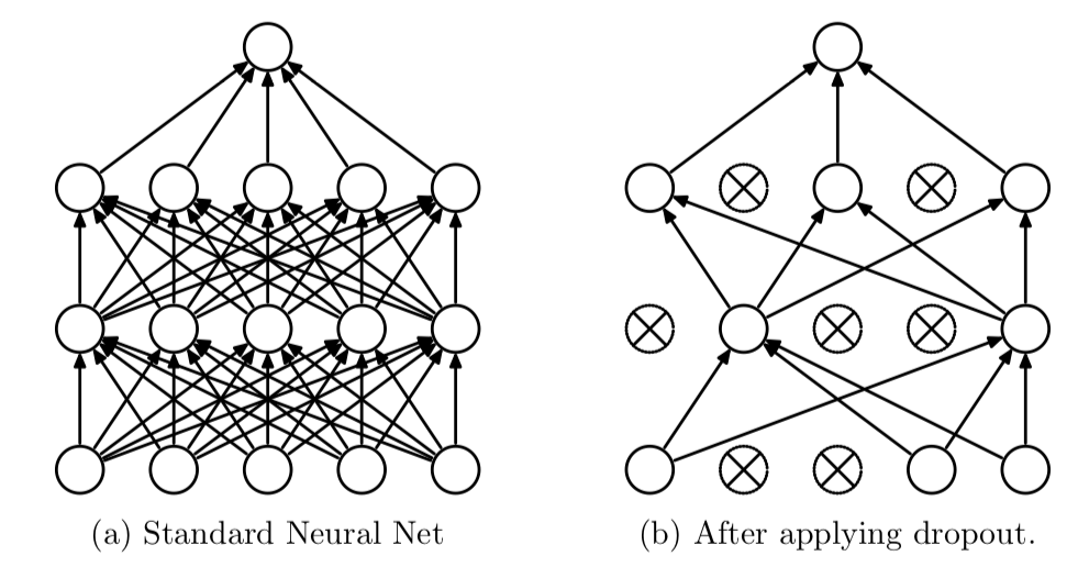
Just like batch normalization, it also has different behavior during training and evaluation.

dropout = nn_dropout(p = 0.5)
dropout(x)

torch_tensor
 0.0000 -3.9488  0.0093  0.0000  0.7024
-0.0000 -1.4141  0.0000  2.9566  5.7694
-4.4366  0.7622 -0.0000  2.1163  0.2118
 0.0000  0.0000  0.0000  0.6584  0.2422
-0.0000 -0.0000 -0.9663 -0.0000 -5.1942
 0.0000 -1.0714  2.3080 -0.0000  0.6326
-1.1987 -5.4360  0.0000  3.8675  0.0000
 0.0000  0.8761  2.7579  3.5069 -0.0000
-0.3855  1.1178 -0.0000  0.8627  0.0000
-0.0000  0.0000  0.0000 -0.0000  1.5217
[ CPUFloatType{10,5} ]

dropout$eval()
dropout(x)

torch_tensor
 0.9281 -1.9744  0.0046  1.7829  0.3512
-1.2553 -0.7071  2.2261  1.4783  2.8847
-2.2183  0.3811 -2.0875  1.0582  0.1059
 0.2226  0.0924  0.5471  0.3292  0.1211
-1.2201 -0.1440 -0.4831 -1.1782 -2.5971
 0.3462 -0.5357  1.1540 -1.1725  0.3163
-0.5994 -2.7180  0.0385  1.9338  0.1908
 0.3669  0.4380  1.3789  1.7534 -0.5429
-0.1927  0.5589 -0.5695  0.4313  0.1367
-0.2556  1.6093  0.2711 -0.4924  0.7609
[ CPUFloatType{10,5} ]

To look at the effects, we will create a second classification head with dropout and then define new learners.

head_dropout = po("nn_flatten") %>>%
  po("nn_linear", out_features = 128) %>>%
  po("nn_relu") %>>%
  po("nn_dropout", p = 0.5) %>>%
  po("nn_head")

net_bn_dropout = as_learner(cnn_bn %>>% head_dropout %>>% model)
net_bn_dropout$id = "net_bn_dropout"
net_dropout = as_learner(cnn %>>% head_dropout %>>% model)
net_dropout$id = "net_dropout"

design2 = benchmark_grid(
  task = cifar10,
  learner = list(net_bn_dropout, net_dropout),
  resampling = resampling
)

Next, we run the second benchmark experiment and afterwards combine the results with the first benchmark experiment.

bmr2 = benchmark(design2)
bmr = c(bmr, bmr2)
autoplot(bmr)

Quiz: Dropout

Question 1: Worse Training Loss: You are training a neural network with and without dropout. The training loss is higher with dropout, is this a bug?

Click for answer

Not necessarily, as dropout is a regularization technique that prevents overfitting. Its goal is to reduce the generalization performance of the model and not to improve training performance.

Transfer Learning

Transfer learning is a powerful technique in machine learning where a pre-trained model developed for a specific task is reused as the starting point for a model on a second, related task. Instead of training a model from scratch, which can be time-consuming and computationally expensive, transfer learning leverages the knowledge gained from a previously learned task to improve learning efficiency and performance on a new task.

The advantages of transfer learning are:

1. Reduced Training Time: Leveraging a pre-trained model can significantly decrease the time required to train a new model, as the foundational feature extraction layers are already optimized.
2. Improved Performance: Transfer learning can enhance model performance, especially when the new task has limited training data. The pre-trained model’s knowledge helps in achieving better generalization.
3. Resource Efficiency: Utilizing pre-trained models reduces the computational resources needed, making it feasible to develop sophisticated models without extensive hardware.

When the model is then trained on a new task, only the last layer is replaced with a new output layer to adjust for the new task.

This is visualized below:

Source

mlr3torch offers various pretrained image networks that are available through the torchvision package. The ResNet-18 model is a popular pre-trained model that was pretrained on ImageNet. We can use the pretrained weights by setting the pretrained parameter to TRUE.

resnet = lrn("classif.resnet18",
  pretrained = TRUE,
  epochs = 2,
  batch_size = 256,
  validate = 0.3,
  measures_valid = msr("classif.logloss"),
  device = "cuda",
  predict_type = "prob",
  id = "pretrained"
)
resnet_no_pretrain = resnet$clone(deep = TRUE)
resnet_no_pretrain$param_set$set_values(
  pretrained = FALSE
)
resnet_no_pretrain$id = "not_pretrained"

grid = benchmark_grid(
  task = tsk("cifar10"),
  learner = list(resnet, resnet_no_pretrain),
  resampling = rsmp("insample")
)

bmr = benchmark(grid, store_models = TRUE)
bmr$aggregate()

When fine-tuning a pretrained model like ResNet-18, it’s common to observe instabilities in gradients, which can manifest as fluctuating validation performance.

To address this, one can for example freeze the pretrained layers (for some epochs) and only train the new output head. In mlr3torch, this can be achieved by using the t_clbk("unfreeze") callback.

In-Context Learning

Large foundation models (such as GPT-4) even allow performing tasks on which they were not pretrained on without any finetuning. This is referred to as in-context learning or zero-shot learning. There, the task is fed into the model during inference: “Hey ChatGPT, is What is the sentiment of this sentence. Return -1 for sad, 0 for neutral, 1 for happy: ”

Data Augmentation

Data augmentation is a technique used to increase the diversity and quantity of training data without actually collecting new data. By applying various transformations to the existing dataset, data augmentation helps improve the generalization capabilities of machine learning models, reduce overfitting, and enhance model robustness. This is especially crucial when you have limited data.

Data augmentation for images can consist of rotation, flipping, translating, grey scaling, etc. Which data augmentation is admissible, depends on the task:

• If the modeling task is to predict whether there is a mark in the top right corner of an image, vertical or horizontal flipping is not admissible.
• If the goal is to predict whether there is a mark somewhere in the image, it would be admissible.

In other words, the data augmentation must be compatible with the invariances of the task.

In mlr3torch, data augmentation is available via PipeOps of the form po("augment_"). Currently, only augmentation operators from the torchvision package are available, but you can also add your own.

augment = po("augment_random_resized_crop") %>>%
  po("augment_random_horizontal_flip") %>>%
  po("augment_random_vertical_flip")

We can just create a new GraphLearner that includes the augmentation steps as well as the learner from above:

resnet_augmented = as_learner(augment %>>% resnet)
resnet_augmented$id = "resnet_augmented"
resnet_augmented$train(task = cifar10)

Quiz: Data Augmentation

Question 1: Do you think data augmentation should be applied to the validation set?

Click for answer

No, as the purpose of data augmentation is not to improve an individual prediction, it will not be applied during test time and hence also not to the validation set. Looking at the performance of augmented validation data is, however, also not a mistake.