In this exercise, the task is to play around with the settings for the optimization of a neural network. We start by generating some (highly non-linear) synthetic data using the mlbench package.
The code to compare different optimizer configurations is provided via the compare_configs() function, which you can copy paste.
Implementation of compare_configs
library(ggplot2)compare_configs <-function(epochs =30, batch_size =16, lr =0.01, weight_decay =0.01, beta1 =0.9, beta2 =0.999) {# Identify which parameter is a list args <-list(batch_size = batch_size, lr = lr, weight_decay = weight_decay, beta1 = beta1, beta2 = beta2) is_list <-sapply(args, is.list)if (sum(is_list) !=1) {stop("One of the arguments must be a list") } list_arg_name <-names(args)[is_list] list_args <- args[[list_arg_name]] other_args <- args[!is_list]# Run train_valid for each value in the list results <-lapply(list_args, function(arg) { network <-with_torch_manual_seed(seed =123, nn_mlp()) other_args[[list_arg_name]] <- argtrain_valid(network, ds_train = ds_train, ds_valid = ds_valid, epochs = epochs, batch_size = other_args$batch_size,lr = other_args$lr, betas =c(other_args$beta1, other_args$beta2), weight_decay = other_args$weight_decay) })# Combine results into a single data frame combined_results <-do.call(rbind, lapply(seq_along(results), function(i) { df <- results[[i]] df$config <-paste(list_arg_name, "=", list_args[[i]]) df })) upper <-if (max(combined_results$valid_loss) >10) quantile(combined_results$valid_loss, 0.98) elsemax(combined_results$valid_loss)ggplot(combined_results, aes(x = epoch, y = valid_loss, color = config)) +geom_line() +theme_minimal() +labs(x ="Epoch", y ="Validation RMSE", color ="Configuration") +ylim(min(combined_results$valid_loss), upper)}train_loop <-function(network, dl_train, opt) { network$train() coro::loop(for (batch in dl_train) { opt$zero_grad() Y_pred <-network(batch[[1]]) loss <-nnf_mse_loss(Y_pred, batch[[2]]) loss$backward() opt$step() })}valid_loop <-function(network, dl_valid) { network$eval() valid_loss <-c() coro::loop(for (batch in dl_valid) { Y_pred <-with_no_grad(network(batch[[1]])) loss <-sqrt(nnf_mse_loss(Y_pred, batch[[2]])) valid_loss <-c(valid_loss, loss$item()) })mean(valid_loss)}train_valid <-function(network, ds_train, ds_valid, epochs, batch_size, ...) { opt <-optim_ignite_adamw(network$parameters, ...) train_losses <-numeric(epochs) valid_losses <-numeric(epochs) dl_train <-dataloader(ds_train, batch_size = batch_size) dl_valid <-dataloader(ds_valid, batch_size = batch_size)for (epoch inseq_len(epochs)) {train_loop(network, dl_train, opt) valid_losses[epoch] <-valid_loop(network, dl_valid) }data.frame(epoch =seq_len(epochs), valid_loss = valid_losses)}
It takes as arguments:
epochs: The number of epochs to train for. Defaults to 30.
batch_size: The batch size to use for training. Defaults to 16.
lr: The learning rate to use for training. Defaults to 0.01.
weight_decay: The weight decay to use for training. Defaults to 0.01.
beta1: The momentum parameter to use for training. Defaults to 0.9.
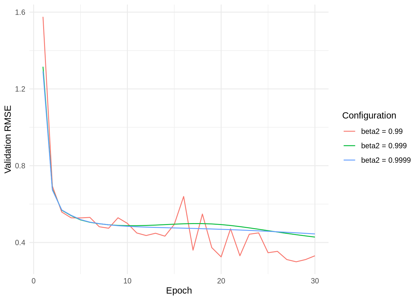
beta2: The adaptive step size parameter to use for training. Defaults to 0.999.
You can, e.g., call the function like below:
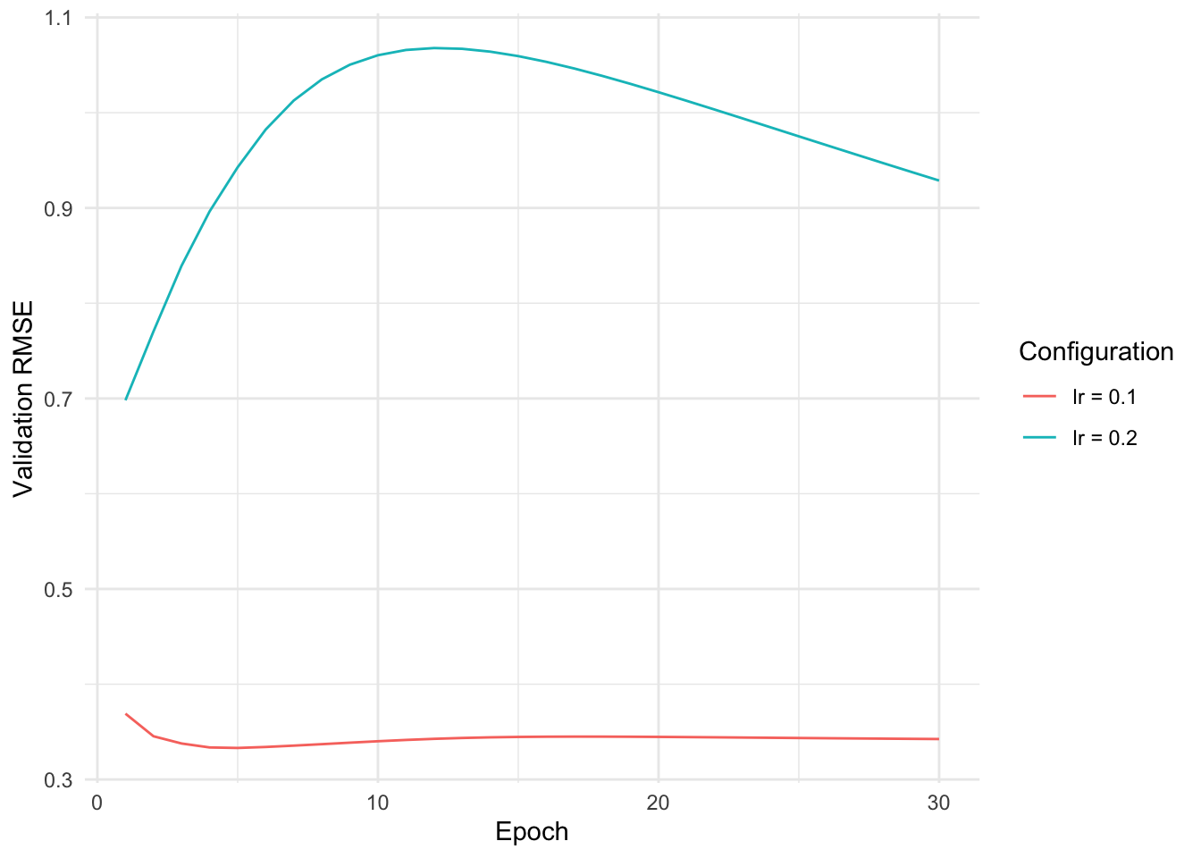
compare_configs(epochs =30, lr =list(0.1, 0.2), weight_decay =0.02)
One of the arguments (except for epochs) must be a list of values. The function will then run the same training configuration for each of the values in the list and visualize the results.
Explore a few hyperparameter settings and make some observations as to how they affect the trajectory of the validation loss. The purpose of this exercise is not to derive observations that hold in general.
Solution
There is not really a ‘solution’ to this exercise. We will go through some of the configurations and try to explain what is happening.
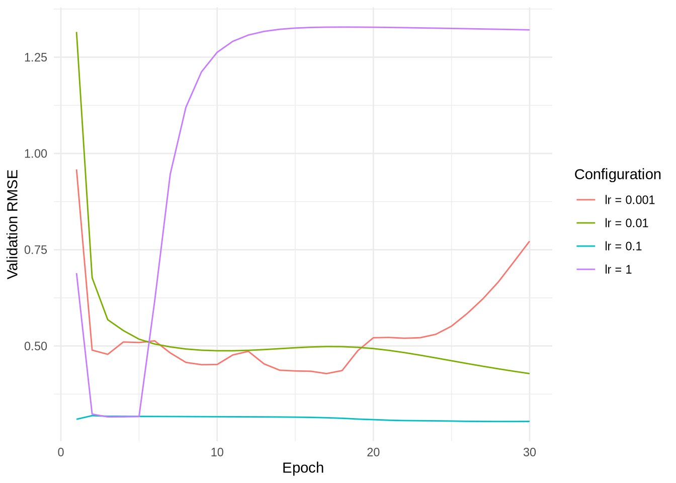
Learning rate
compare_configs(epochs =30, lr =list(1, 0.1, 0.01, 0.001))
Too large learning rates lead to unstable updates and divergence. It is not exactly clear why the small learning rate is so unstable, possibly it gets stuck in a bad region of the loss landscape.
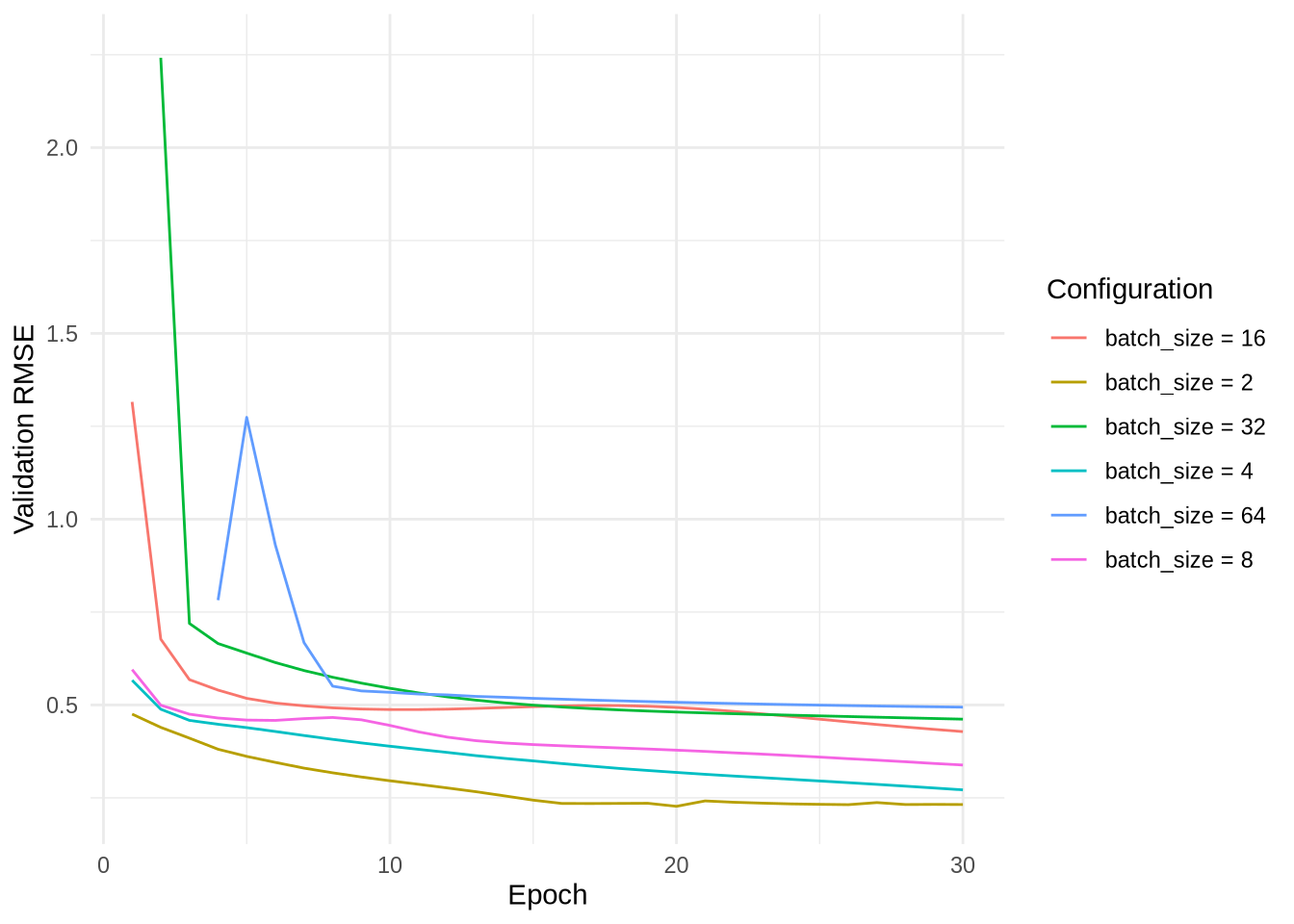
Batch Size
For this configuration, we can see that smaller batch sizes lead to considerably better results as they allow for more updates for the given number of epochs.
Note that this comparison is not entirely fair as the number of epochs is fixed. We would rather be interested in the performance of different batch sizes for a fixed amount of time and not epochs.
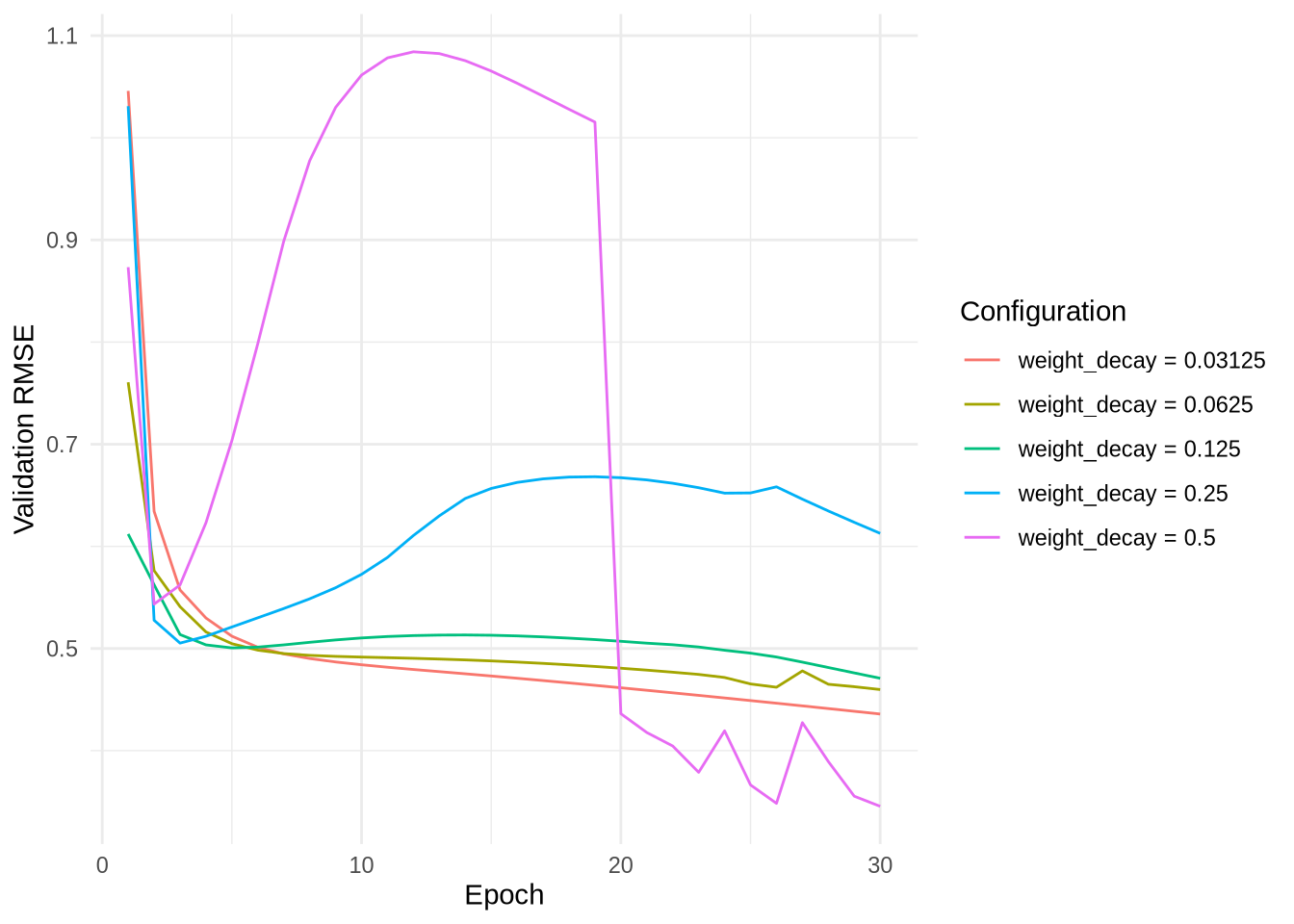
Weight Decay
For too large values of the weight decay, we see that the network struggles to get a good validation loss at first.
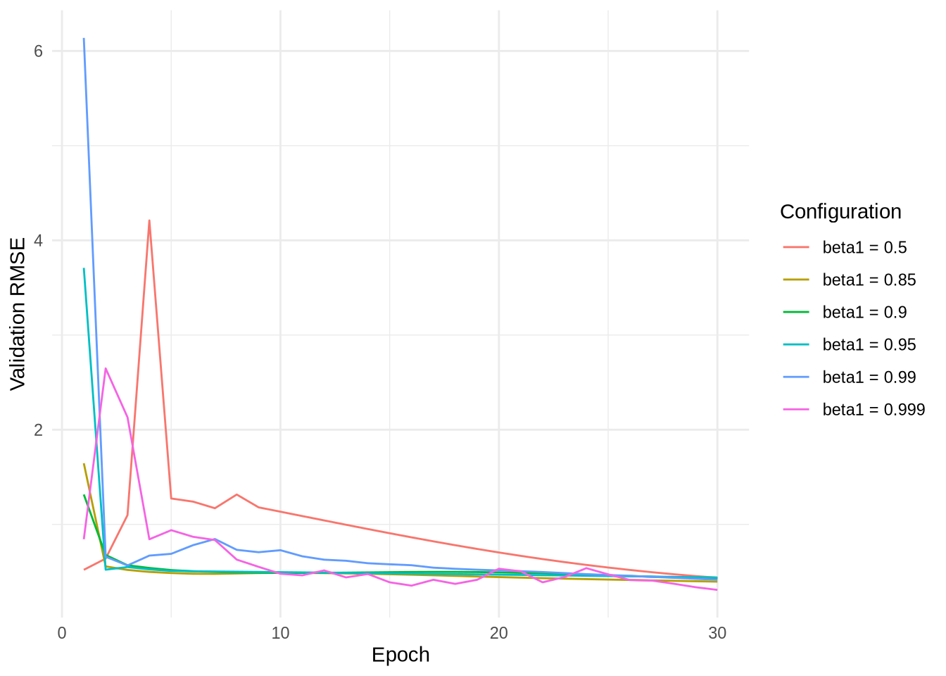
We can observe that too large values for the momentum parameter lead to oscillations, possibly because the local information is not used enough. Too small values lead to worse performance.
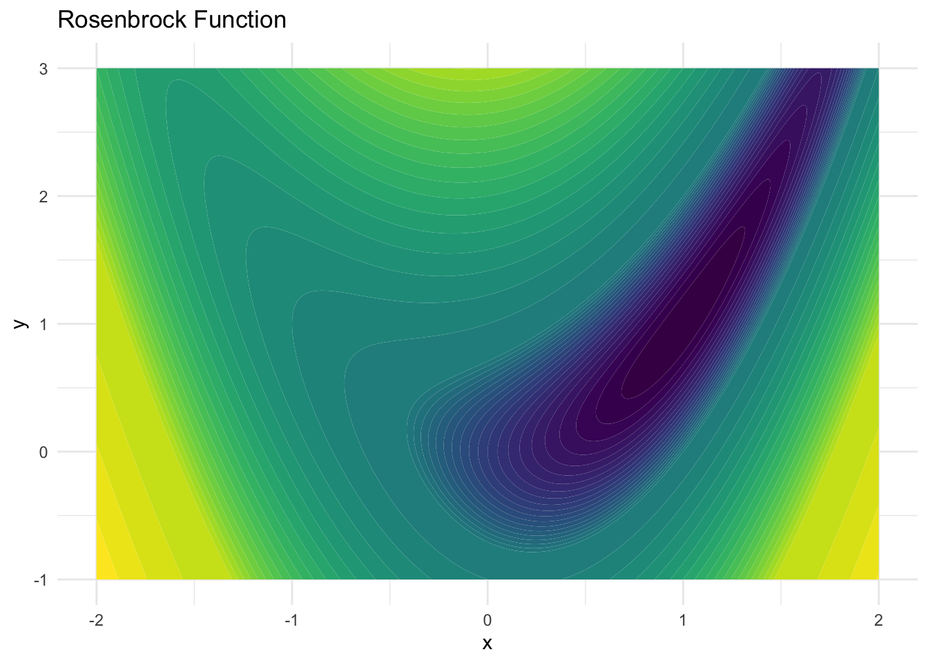
In this exercise, you will build a (simplified) gradient descent optimizer with momentum. As a use case, we will minimize the Rosenbrock function. The function is defined as:
The ‘parameters’ we will be optimizing is the position of a point (x, y), which will both be updated using gradient descent. The figure below shows the Rosenbrock function, where darker values indicate lower values.
The task is to implement the optim_step() function.
optim_step <-function(x, y, lr, x_momentum, y_momentum, beta) { ...}
It will receive as arguments, the current values x and y, the momentum values x_momentum and y_momentum (all scalar tensors) as well as the learning rate lr and the momentum parameter beta. The function should then:
Perform a forward pass.
Calculate the gradients.
Update the momentum values in-place.
Update the parameters in-place.
Hint
To perform in-place updates, you can use the $mul_() and $add_() methods.
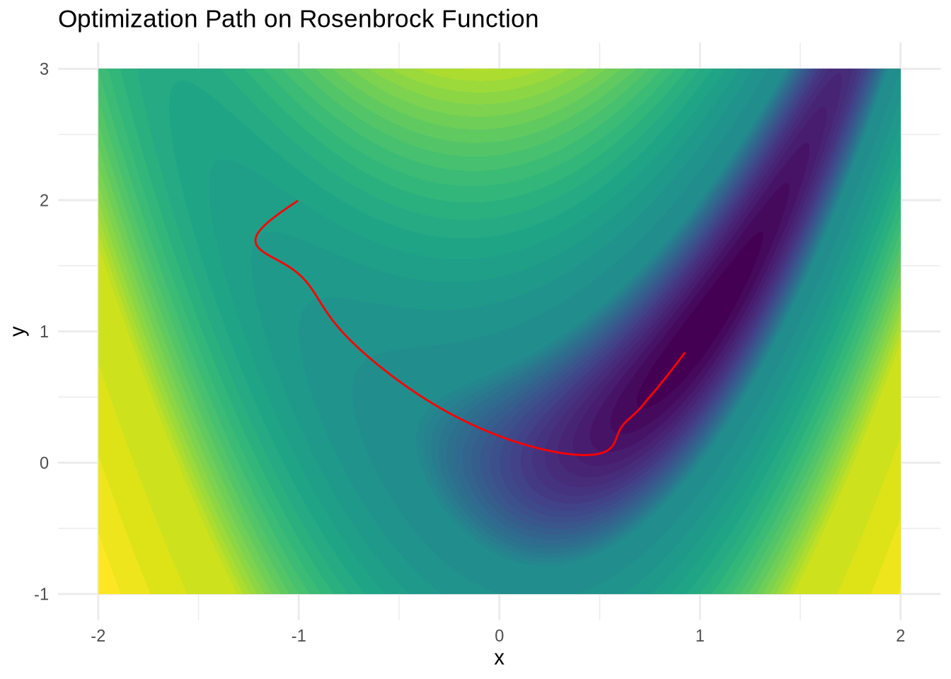
To test your optimizer, you can use the code below. Note that you might have to play around with the number of steps and the learning rate to get a good result.
Code to test your optimizer
x <-seq(-2, 2, length.out =400)y <-seq(-1, 3, length.out =400)grid <-expand.grid(x = x, y = y)grid$z <-with(grid, rosenbrock(x, y))breaks <-c(seq(0, 1.9, by =0.1), seq(2, 19, by =1), seq(20, 190, by=10), seq(200, 2000, by =200))plot_rosenbrock <-function() {ggplot(grid, aes(x = x, y = y, z = z)) +geom_contour_filled(breaks = breaks) +labs(title ="Rosenbrock Function", x ="x", y ="y") +theme_minimal() +theme(legend.position ="none")}optimize_rosenbrock <-function(steps, lr, beta) { x <-torch_tensor(-1, requires_grad =TRUE) y <-torch_tensor(2, requires_grad =TRUE) momentum_x <-torch_tensor(0) momentum_y <-torch_tensor(0) trajectory <-data.frame(x =numeric(steps +1),y =numeric(steps +1),value =numeric(steps +1) )for (step inseq_len(steps)){optim_step(x, y, lr, momentum_x, momentum_y, beta) x$grad$zero_() y$grad$zero_() trajectory$x[step] <- x$item() trajectory$y[step] <- y$item() } trajectory$x[steps +1] <- x$item() trajectory$y[steps +1] <- y$item()plot_rosenbrock() +geom_path(data = trajectory, aes(x = x, y = y, z =NULL), color ="red") +labs(title ="Optimization Path on Rosenbrock Function", x ="x", y ="y")}
In exercise 2, we have optimized the Rosenbrock function. Does it make sense to also use weight decay here?
Solution No, it does not make sense to use weight decay for this optimization as it is intended to prevent overfitting which is not a problem in this case. This is, because there is no uncertainty in the function we are optimizing.