Autograd

Question 1: Appreciating autograd

Consider the following function:

\[ f(x) = x^2 + 3x + 2 \]

As well as the function $g(x) = f(f(f(x)))$

Calculate the gradient of both functions at point $x = 2$.

Solution

library(torch)
x <- torch_tensor(2, requires_grad = TRUE)
f <- function(x) {
  x^2 + 3 * x + 2
}
g <- function(x) {
  f(f(f(x)))
}

# Calculate f'(2)
f(x)$backward()
grad <- x$grad$clone()
grad

torch_tensor
 7
[ CPUFloatType{1} ]

# For another backward pass, we reset the gradient as they otherwise accumulate
x$grad$zero_()

torch_tensor
 0
[ CPUFloatType{1} ]

# Calculate the gradient of g(x)
g(x)$backward()

# Create a copy of the gradient
grad2 <- x$grad$clone()
grad2

torch_tensor
 69363
[ CPUFloatType{1} ]

# Zero gradients for good measure
x$grad$zero_()

torch_tensor
 0
[ CPUFloatType{1} ]

Question 2: Approximating functions with gradients

The defining feature of the gradient is that it allows us to approximate the function locally by a linear function.

I.e., for some value $x^*$, we know for very small $\delta$, that

\[ f(x^* + \delta) \approx f(x^*) + f'(x^*) \cdot \delta \]

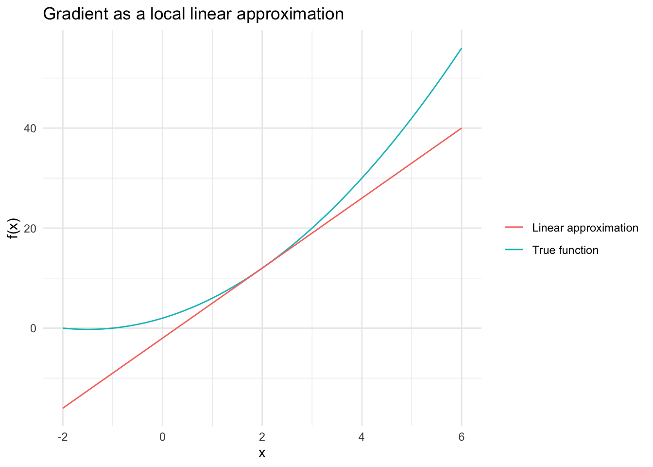
Plot the function from earlier as well as the local linear approximation at $x = 2$ using ggplot2.

Hint

To do so, follow these steps:

Create a sequence with 100 equidistant values between -4 to 4 using torch_linspace().
Create the true function values at these points using the function from exercise 1.
Approximate the function using the formula $f(x^* + \delta) \approx f(x^*) + f'(x^*) \cdot \delta$.
Create a data.frame with columns x, y_true, y_approx.
Use ggplot2 to plot the function and its linear approximation.

Solution

library(ggplot2)
x <- x$detach() # No need to track gradients anymore
deltas <- torch_linspace(-4, 4, 100)
y_true <- f(x + deltas)
y_approx <- f(x) + grad * deltas

d <- data.frame(x = as_array(x + deltas), y_true = as_array(y_true), y_approx = as_array(y_approx))

ggplot(d, aes(x = x)) +
  geom_line(aes(y = y_true, color = "True function")) +
  geom_line(aes(y = y_approx, color = "Linear approximation")) +
  theme_minimal() +
  labs(
    title = "Gradient as a local linear approximation",
    y = "f(x)",
    x = "x",
    colour = ""
  )

Question 3: Look ma, I made my own autograd function

In this exercise, we will build our own, custom autograd function. While you might rarely need this in practice, it still allows you to get a better understanding of how the autograd system works. There is also a tutorial on this on the torch website.

To construct our own autograd function, we need to define:

The forward pass:
- How to calculate outputs from input
- What to save for the backward pass
The backward pass:
- How to calculate the gradient of the output with respect to the input

The task is to re-create the ReLU activation function, which is a common activation function in neural networks and which is defined as:

\[ \text{ReLU}(x) = \max(0, x) \]

Note that strictly speaking, the ReLU function is not differentiable at $x = 0$ (but a subgradient can be used instead). The derivative/subgradient of the ReLU function is:

\[ \text{ReLU}'(x) = \begin{cases} 1 & \text{if } x > 0 \\ 0 & \text{if } x \leq 0 \\ \end{cases} \]

In torch, a custom autograd function can be constructed using autograd_function() and it accepts arguments forward and backward which are functions that define the forward and backward pass: They both take as first argument a ctx, which is a communication object that is used to save information during the forward pass to be able to compute the gradient in the backward pass (e.g. for $f(x) = x * a$, to calculate the gradient of $f$ with respect to $a$ we need to know the input value $x$). The return value of the backward pass should be a list of gradients with respect to the inputs. To check whether a gradient for an input is needed (has requires_grad = TRUE), you can use ctx$needs_input_grad which is a named list with boolean values for each input.

The backward function additionally takes a second argument grad_output, which is the gradient of the output: E.g., if our function is $f(x)$ and we calculate the gradient of $g(x) = h(f(x))$, then grad_output is the derivative of $g$ with respect to its input, evaluated at $f(x)$. This is essentially the chain rule: $\frac{\partial g}{\partial x} = \frac{\partial h}{\partial f} \cdot \frac{\partial f}{\partial x}$.

Fill out the missing parts (...) in the code below.

relu <- autograd_function(
  forward = function(ctx, input) {
    mask <- ...
    output <- torch_where(mask, ...)
    ctx$save_for_backward(mask)
    output
  },
  backward = function(ctx, grad_output) {
    grads <- list(input = NULL)
    if (ctx$needs_input_grad$input) {
      mask <- ctx$saved_variables[[1]]
      grads$input <- ...
    }
    grads
  }
)

To check that it’s working, use the code below (with your relu instead of nnf_relu) and check that the results are the same.

x <- torch_tensor(-1, requires_grad = TRUE)
(nnf_relu(x)^2)$backward()
x$grad

torch_tensor
 0
[ CPUFloatType{1} ]

x$grad$zero_()

torch_tensor
 0
[ CPUFloatType{1} ]

x <- torch_tensor(3, requires_grad = TRUE)
(nnf_relu(x)^2)$backward()
x$grad

torch_tensor
 6
[ CPUFloatType{1} ]

Solution

relu <- autograd_function(
  forward = function(ctx, input) {
    mask <- input > 0
    output <- torch_where(mask, input, torch_tensor(0))
    ctx$save_for_backward(mask)
    output
  },
  backward = function(ctx, grad_output) {
    grads <- list(input = NULL)
    if (ctx$needs_input_grad$input) {
      mask <- ctx$saved_variables[[1]]
      grads$input <- grad_output * mask
    }
    grads
  }
)

x <- torch_tensor(-1, requires_grad = TRUE)
(relu(x)^2)$backward()
x$grad

torch_tensor
 0
[ CPUFloatType{1} ]

x$grad$zero_()

torch_tensor
 0
[ CPUFloatType{1} ]

x <- torch_tensor(3, requires_grad = TRUE)
(relu(x)^2)$backward()
x$grad

torch_tensor
 6
[ CPUFloatType{1} ]