Question 1: Create a torch::dataset class that takes in arguments n, min, and max during initialization where:
n is the total number of samples
min is the lower bound of the data
max is the upper bound of the data
In the initialize method, generate and store:
a tensor x of shape (n, 1) that contains n values drawn from a uniform distribution between min and max
a tensor y of shape (n, 1) that is defined as \(\sin(x) + \epsilon\) where \(\epsilon\) is drawn from a normal distribution with mean 0 and standard deviation 0.1
Hint
Use torch_randn() to draw from a standard normal distribution and multiply it with 0.1^2 to get the desired standard deviation.
Implement the $.getbatch() method to return a named list with values x and y. Then, create an instance of the dataset with n = 1000, min = 0, and max = 10.
Make sure that the dataset is working by calling the $.getbatch() method. Also, check that the shapes of both tensors returned by the dataset are (n_batch, 1).
Solution
library(torch)sin_dataset <-dataset(initialize =function(n, min, max) { self$x <-torch_rand(n, 1) * (max - min) + min self$y <-torch_sin(self$x) +torch_randn(n, 1) *0.1^1 },.getbatch =function(i) {list(x = self$x[i, drop =FALSE], y = self$y[i, drop =FALSE]) },.length =function() {length(self$x) })ds <-sin_dataset(n =1000, min =0, max =10)batch <- ds$.getbatch(1:10)batch$x$shape
[1] 10 1
batch$y$shape
[1] 10 1
Question 2: Create a torch::dataloader that takes in the dataset and returns batches of size 10. Then, iterate over the batches of the dataloader and create one tensor X and one tensor Y that contains the concatenated batches of x and y.
Hint
The functions coro::loop() and torch_cat() might be helpful.
Solution
dl <-dataloader(ds, batch_size =10)batches <-list()coro::loop(for (batch in dl) { batches <-c(batches, list(batch))})X <-torch_cat(lapply(batches, function(batch) batch$x), dim =1)X$shape
[1] 1000 1
Y <-torch_cat(lapply(batches, function(batch) batch$y), dim =1)Y$shape
[1] 1000 1
Question 3: Create a custom torch module that allows modeling the sinus data we have created. To test it, apply it to the tensor X we have created above and calculate its mean squared error with the tensor Y. Don’t forget to run it without tracking gradients.
Hint
You can either use nn_module to create a custom module generically, or you can use nn_sequential() to create a custom module that is a sequence of layers.
Question 4: Train the model on the task for different hyperparameters (lr or epochs) and visualize the results. Play around with the hyperparameters until you get a good fit. You can use the following code for that:
library(ggplot2)predict_network <-function(net, dataloader) {local_no_grad() xs <-list(x =numeric(), y =numeric(), pred =numeric()) i <-1 net$eval() coro::loop(for (batch in dataloader) { xs$x <-c(xs$x, as.numeric(batch$x)) xs$y <-c(xs$y, as.numeric(batch$y)) xs$pred <-c(xs$pred, as.numeric(net(batch$x))) })as.data.frame(xs)}train_network <-function(net, dataloader, epochs, lr) { optimizer <-optim_ignite_adamw(net$parameters, lr = lr) net$train()for (i inseq_len(epochs)) { coro::loop(for (batch in dataloader) { optimizer$zero_grad() Y_pred <-net(batch$x) loss <-nnf_mse_loss(Y_pred, batch$y) loss$backward() optimizer$step() }) }predict_network(net, dataloader)}plot_results <-function(df) {ggplot(data = df, aes(x = x)) +geom_point(aes(y = y, color ="true")) +geom_point(aes(y = pred, color ="pred")) +theme_minimal() +labs(color ="")}train_and_plot <-function(net, dataloader, epochs =10, lr =0.01) { result <-train_network(net, dataloader, epochs = epochs, lr = lr)plot_results(result)}
Tip
Beware of the reference semantics and make sure that you create a new instance of the network for each run.
Solution
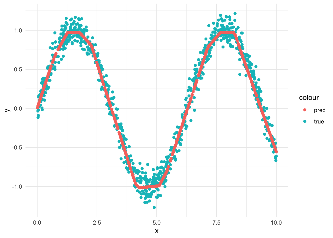
net <-nn_sin(200)train_and_plot(net, dl, epochs =200, lr =0.01)
Question 5: Create a new instance from the sinus dataset class created earlier. Now, set the min and max values to 10 and 20 respectively and visualize the predictions of the previously trained network on this new dataset. What do you observe? Can you explain why this is happening and can you fix the network architecture to make it work?
Hint
The sinus function has a phase of \(2 \pi\).
Solution
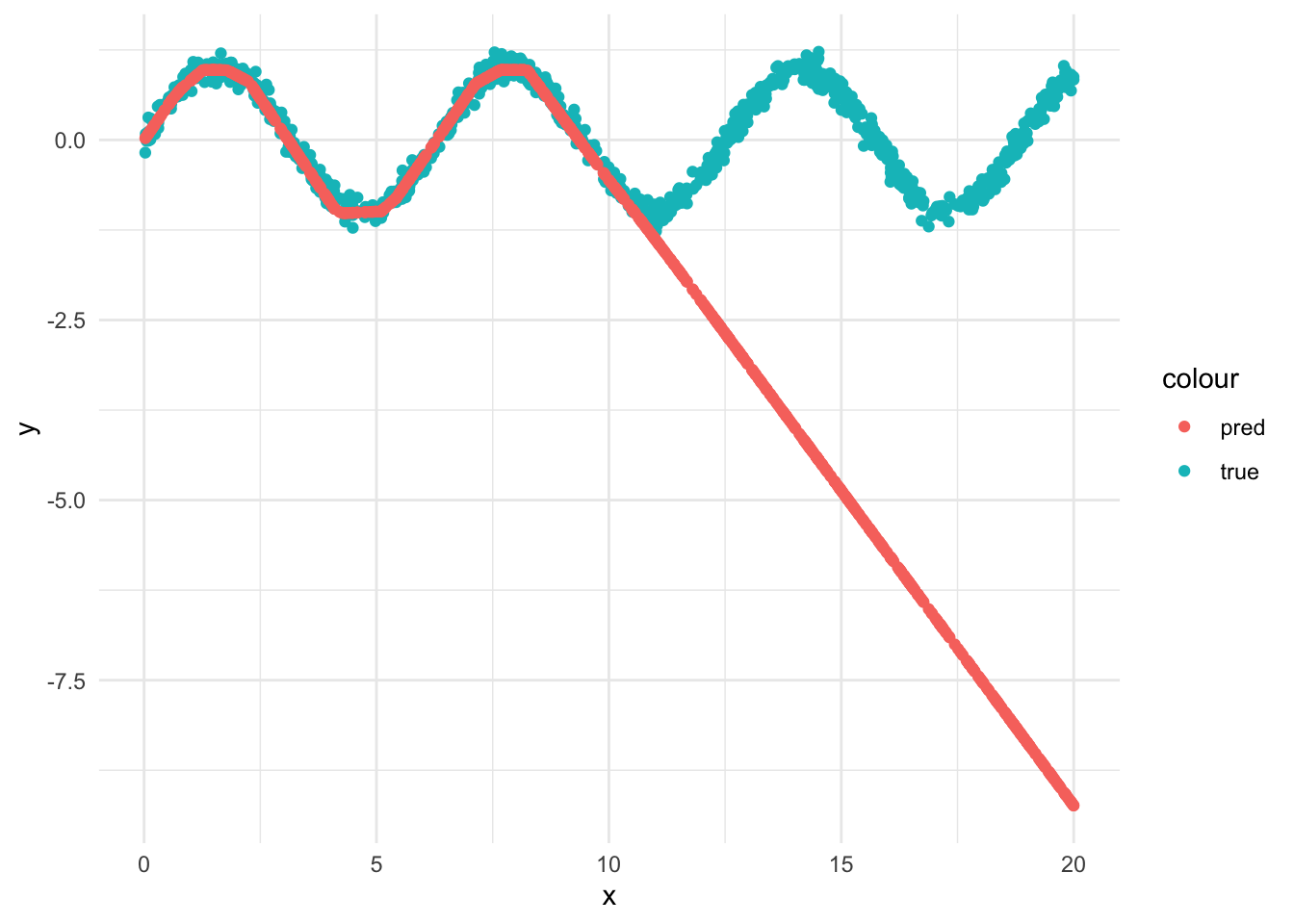
dl_ood <-dataloader(sin_dataset(n =1000, min =0, max =20), batch_size =10)plot_results(predict_network(net, dl_ood))
For values in the range [10, 20], the network fails to generalize. This is because the network only observed values in the range [0, 10] during training.
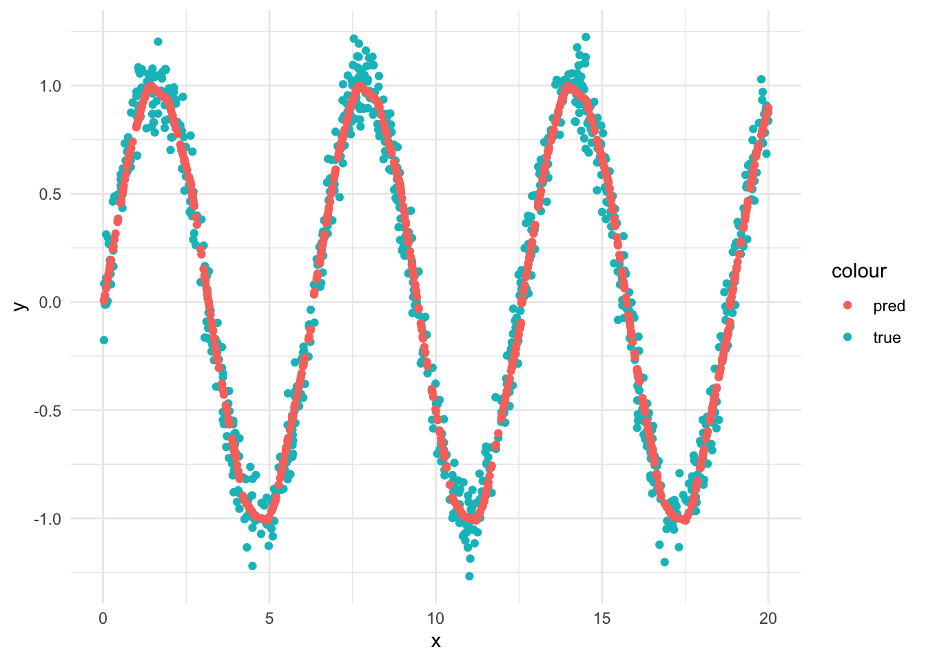
We can fix this by preprocessing the data using the modulo operator, i.e. using the correct inductive bias for the problem.