Convolutional Neural Networks
In this notebook, we explore convolutional neural networks (CNNs) used for image classification tasks. Image classification is fundamentally different from working with tabular data because images are highly structured and high-dimensional. For example, in an image, nearby pixels have strong spatial dependencies, whereas tabular data typically consists of independent or loosely related features, with each column representing a distinct attribute.
Convolutional Layers
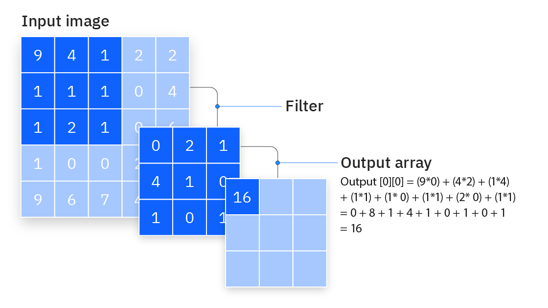
The central component of a CNN is the convolutional layer. It functions by sliding a kernel over the input image, performing element-wise multiplication with the overlapping pixel values, and summing the results to produce a single output value for each kernel position.
CNNs incorporate several strong inductive biases about visual data:
- Locality: Nearby pixels are more likely to be related than distant ones.
- Translation Invariance: Features should be detected regardless of their position.
These biases make CNNs particularly effective for image-related tasks, as they align with our understanding of how visual information is structured.
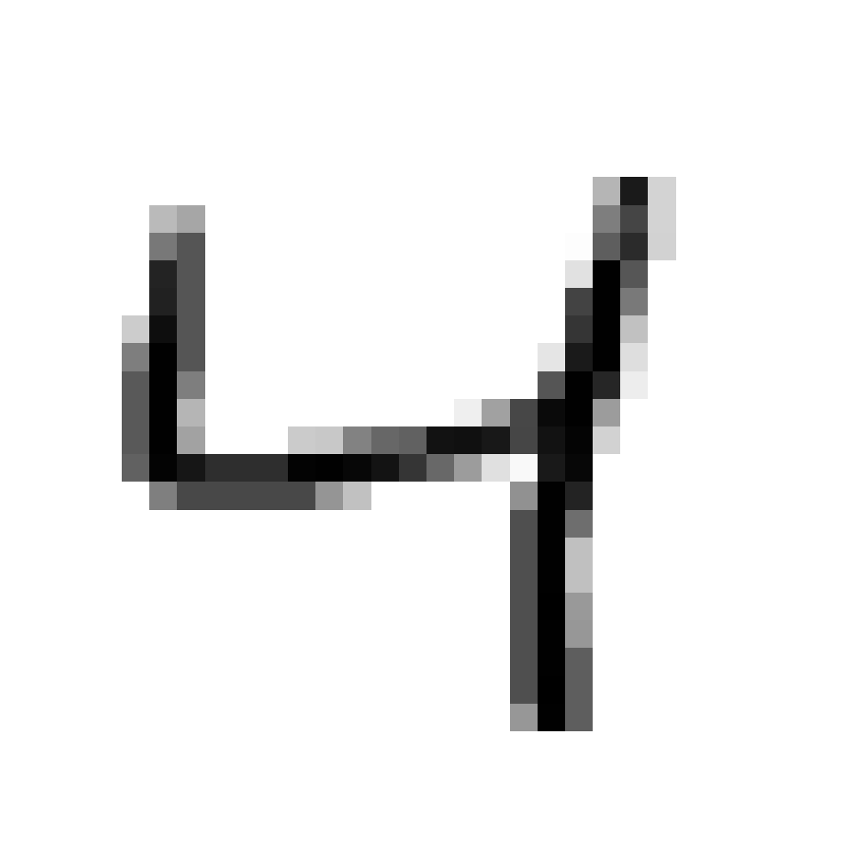
As a first example, we will apply a convolutional layer to an image from MNIST—a benchmark dataset widely used in the machine learning community. MNIST comprises 28×28 grayscale images of handwritten digits (ranging from 0 to 9). The classification task is to assign the correct digit to each image.
When working with these images as tensors, each is represented a 3D tensor with dimensions [1, 28, 28], where the first dimension are the number of channels (would be 3 for RGB images, but MNIST is grayscale), and the other two dimensions are the spatial dimensions (width and height) of the image.
str(image)Float [1:1, 1:28, 1:28]A convolutional layer has the following parameters:
- in_channels: The number of channels in the input image (e.g., 1 for grayscale images and 3 for RGB images).
- out_channels: The number of filters (or kernels) used by the layer. This determines the number of channels in the output.
- kernel_size: The size of the filter that moves over the image. For instance, a kernel size of 3 means a 3×3 filter.
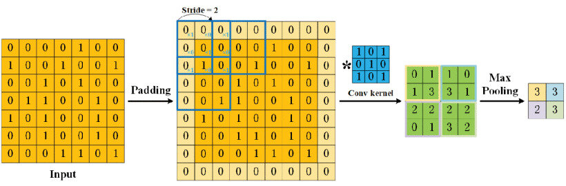
- padding: The number of pixels added to the borders of the input image. Padding can help control the spatial dimensions of the output.
- stride: The step size with which the filter moves across the input image. A larger stride results in a smaller output feature map.
The padding and the strides are visualized below:
To create a convolutional layer for a 2D image, we can use the torch::nn_conv2d function.
conv_layer <- nn_conv2d(in_channels = 1, out_channels = 1, kernel_size = 3, padding = 1, stride = 1)
str(conv_layer(image))
Float [1:1, 1:28, 1:28]
Parameters of a Convolutional Layer
Question 1: Can you set the number of input channels of a convolutional layer freely?
Click for answer
No, the number of input channels is determined by the number of channels of the input tensor.Question 2: Can you come up with a formula for the number of parameters of a convolutional layer? You can assume a symmetric kernel. Note that each kernel also has a bias term which is a scalar.
Click for answer
The formula isout_channels * (kernel_size^2 * in_channels + 1).
Question 3: We have an input image of shape (1, 28, 28) and we want to apply a fully connected layer and a convolutional layer that produces an output tensor with the same number of elements.
- A convolutional layer with 1 input channel and 1 ouput channel and a kernel of size 3x3 and padding of 1. (The output shape will therefore be
(1, 28, 28).) - A fully connected layer (that treats the input as a vector of dimension
28 * 28 = 784) that produces an output tensor with the same number of elements.
How many parameters does each layer have? (Recall that the linear layer also has a bias term.)
Click for answer
- \(1 \times (3 \times 3 \times 1 + 1) = 10\)
- \(784 \times (784 + 1) = 615440\)
Because we have encoded more information about the structural relationship between the input tensor and the output tensor (the same filter is applied to the entire image), the convolutional layer has far fewer parameters than a fully connected layer.
conv_layer$parameters$weight
torch_tensor
(1,1,.,.) =
-0.1359 0.0110 -0.1656
0.1257 -0.2840 0.2443
-0.2423 -0.2650 -0.2106
[ CPUFloatType{1,1,3,3} ][ requires_grad = TRUE ]
$bias
torch_tensor
0.1510
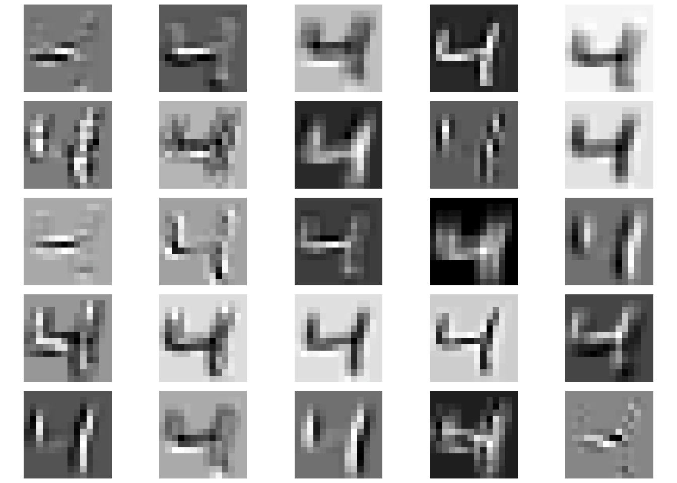
[ CPUFloatType{1} ][ requires_grad = TRUE ]Below, we show the output of the first convolutional layer from a (trained) ResNet18 model applied to an image from MNIST.
Max Pooling
While convolutional layers extract local features from an image by applying a kernel over the input, max pooling is used to downsample the feature maps. Instead of applying a filter, max pooling simply partitions the input into non-overlapping (or sometimes overlapping) regions and selects the maximum value from each region.

Below, we demonstrate it in action and compare the output of a convolutional layer with the results of applying a 2x2 max pooling operation with stride 2 to it.
# Create a max pooling layer with a 2x2 kernel and stride 2
pool_layer <- nn_max_pool2d(kernel_size = 2, stride = 2)

# Now apply the max pooling layer to one channel of the output from the convolution.
pooled_output <- pool_layer(conv_output[1, drop = FALSE]$unsqueeze(1))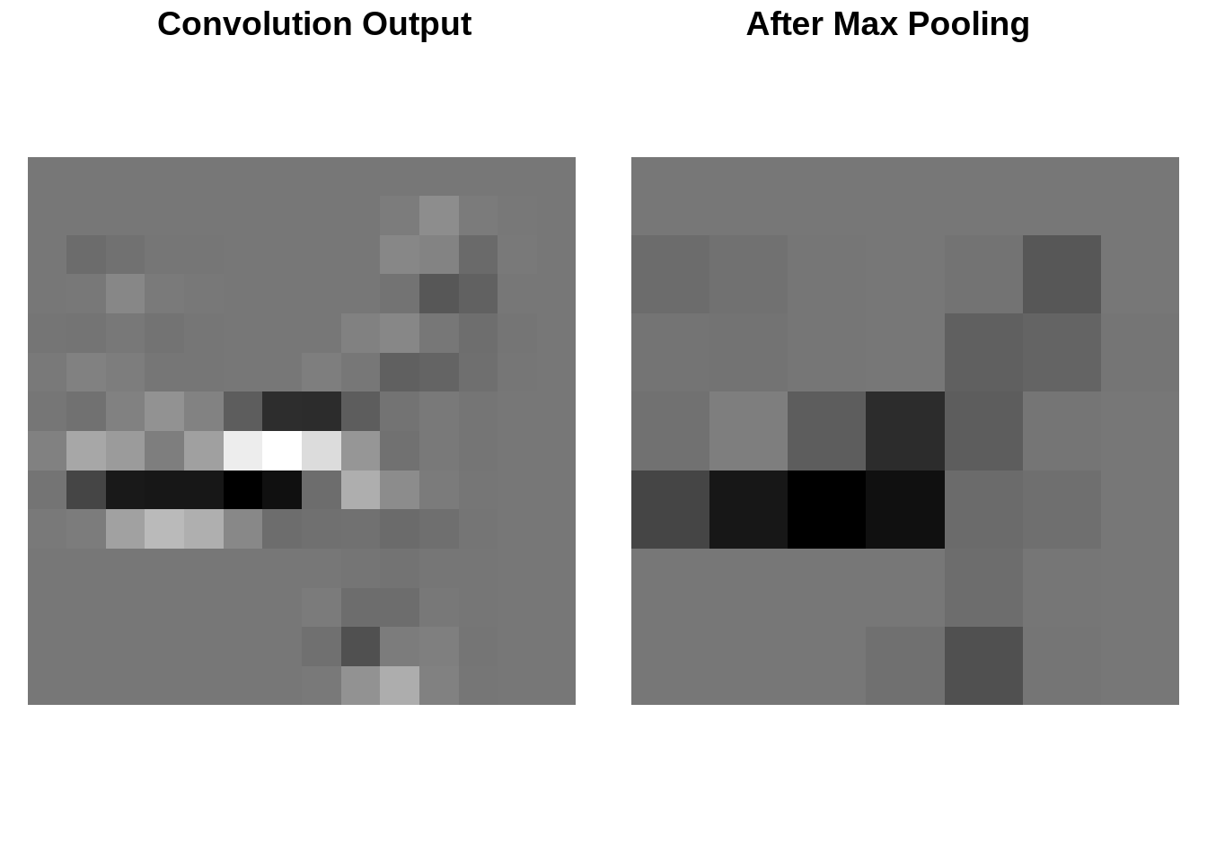
Max Pooling
Question 1: How many parameters does a max pooling layer have?
Click for answer
A max pooling layer has no parameters.Question 2: When applying a max pooling layer to an image of shape (1, 28, 28) and a kernel size of 10x10, a stride of 1 and a padding of 0, what is the shape of the output?
Click for answer
The output shape is(1, 19, 19).
Architecture & Transfer Learning
While we have now covered individual components of CNNs, the question of how to configure and compose them is a challenging task, but essential for building efficient neural networks. However, for many problems, there are predefined architectures that perform well and can be used. Unless there is a specific reason to design a new architecture, it is recommended to use an established one.
Note
Because the Python deep learning ecosystem is so large, many more architectures are implemented in Python than in R. One way to use them in R is to simply translate the PyTorch code to (R-)torch. While PyTorch and (R-)torch are quite similar, there are some differences, e.g., 1-based and 0-based indexing. The torch website contains a brief tutorial on this topic.
Beyond just using a predefined architecture, it is also possible to use transfer learning, which is a powerful technique in machine learning where a pre-trained model developed for a specific task is reused as the starting point for a model on a second, related task. Instead of training a model from scratch, which can be time-consuming and computationally expensive, transfer learning leverages the knowledge gained from a previously learned task to improve learning efficiency and performance on a new task.
The advantages of transfer learning are:
- Reduced Training Time: Leveraging a pre-trained model can significantly decrease the time required to train a new model, as the foundational feature extraction layers are already optimized.
- Improved Performance: Transfer learning can enhance model performance, especially when the new task has limited training data. The pre-trained model’s knowledge helps in achieving better generalization.
- Resource Efficiency: Utilizing pre-trained models reduces the computational resources needed, making it feasible to develop sophisticated models without extensive hardware.
When the model is then trained on a new task, only the last layer is replaced with a new output layer to adjust for the new task.
This is visualized below:
![]()
The torchvision package offers various pretrained image networks that are available through the torchvision package. The ResNet-18 model is a well-known model that was trained on ImageNet. Because it’s architecture is quite complex, we only visualize it below, but don’t define it from scratch.
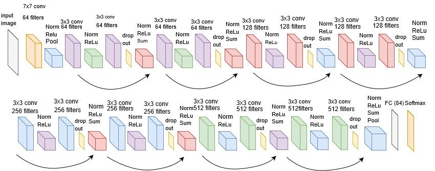
We can access the ResNet-18 model via torchvision and can obtain the pretrained weights by setting the pretrained parameter to TRUE and specifying the number of classes of our new task via the num_classes parameter (10 for MNIST).
library(torchvision)
resnet <- model_resnet18(pretrained = FALSE, num_classes = 10)
resnet_pretrained <- model_resnet18(pretrained = TRUE)
resnet_pretrained$fc <- nn_linear(512, 10)

resnet_pretrained
An `nn_module` containing 11,181,642 parameters.
── Modules ─────────────────────────────────────────────────────────────────────────────────────────────────────────────
• conv1: <nn_conv2d> #9,408 parameters
• bn1: <nn_batch_norm2d> #128 parameters
• relu: <nn_relu> #0 parameters
• maxpool: <nn_max_pool2d> #0 parameters
• layer1: <nn_sequential> #147,968 parameters
• layer2: <nn_sequential> #525,568 parameters
• layer3: <nn_sequential> #2,099,712 parameters
• layer4: <nn_sequential> #8,393,728 parameters
• avgpool: <nn_adaptive_avg_pool2d> #0 parameters
• fc: <nn_linear> #5,130 parametersTo fine-tune this model on MNIST, we need to also have a dataloader. In the case of MNIST, a predefined dataset is available in the torchvision package. We transform both the input and the target to tensors (instead of R arrays).
mnist_ds <- mnist_dataset(root = "data", download = TRUE,
  transform = torch_tensor, target_transform = torch_tensor)
mnist_ds
<mnist>
Inherits from: <dataset>
Public:
.getitem: function (index)
.length: function ()
check_exists: function ()
classes: 0 - zero 1 - one 2 - two 3 - three 4 - four 5 - five 6 - ...
clone: function (deep = FALSE)
data: 0 0 0 0 0 0 0 0 0 0 0 0 0 0 0 0 0 0 0 0 0 0 0 0 0 0 0 0 ...
download: function ()
initialize: function (root, train = TRUE, transform = NULL, target_transform = NULL,
load_state_dict: function (x, ..., .refer_to_state_dict = FALSE)
processed_folder: active binding
raw_folder: active binding
resources: list
root_path: data
state_dict: function ()
target_transform: function (data, dtype = NULL, device = NULL, requires_grad = FALSE,
targets: 6 1 5 2 10 3 2 4 2 5 4 6 4 7 2 8 3 9 7 10 5 1 10 2 2 3 5 ...
test_file: test.rds
train: TRUE
training_file: training.rds
transform: function (data, dtype = NULL, device = NULL, requires_grad = FALSE, We can inspect the first two elements of the dataset.
batch <- mnist_ds[1:2]
str(batch)
List of 2
$ x:Long [1:2, 1:28, 1:28]
$ y:Long [1:2]In order to be able to fine-tune the pretrained model on MNIST, we need to make sure that the format of the input data is compatible with the pretrained model:
- The size of the training images of ResNet-18 were 224x224, while MNIST images are 28x28. We therefore need to resize them.
- ResNet-18 was pretrained on ImageNet, which uses RGB images (3 input channels), while MNIST is grayscale (1 input channel).
- The training images of ResNet-18 were first transformed to be in the range of \([0, 1]\) and then normalized to have a mean of \([0.485, 0.456, 0.406]\) and a standard deviation of \([0.229, 0.224, 0.225]\). Our MNIST images are integer values in the range of \([0, 255]\) so we need to apply both transformations.
We can address this my modifying the transformation from earlier. If we were to implement our own dataset, this would simply be part of the $.getitem() or $.getbatch() method.
transform_mnist <- function(x) {
  x <- torch_tensor(x) / 255
  x <- x$unsqueeze(1)
  x <- x$expand(c(3, 28, 28))
  x <- transform_normalize(x, mean = c(0.485, 0.456, 0.406), std = c(0.229, 0.224, 0.225))
  x <- transform_resize(x, c(224, 224))
  x
}
mnist_train <- mnist_dataset(root = "data", download = TRUE, train = TRUE,
  transform = transform_mnist, target_transform = torch_tensor
)
mnist_test <- mnist_dataset(root = "data", download = TRUE, train = FALSE,
  transform = transform_mnist, target_transform = torch_tensor)
Below, we compare compare the results of training the pretrained and randomly initialized ResNet-18.
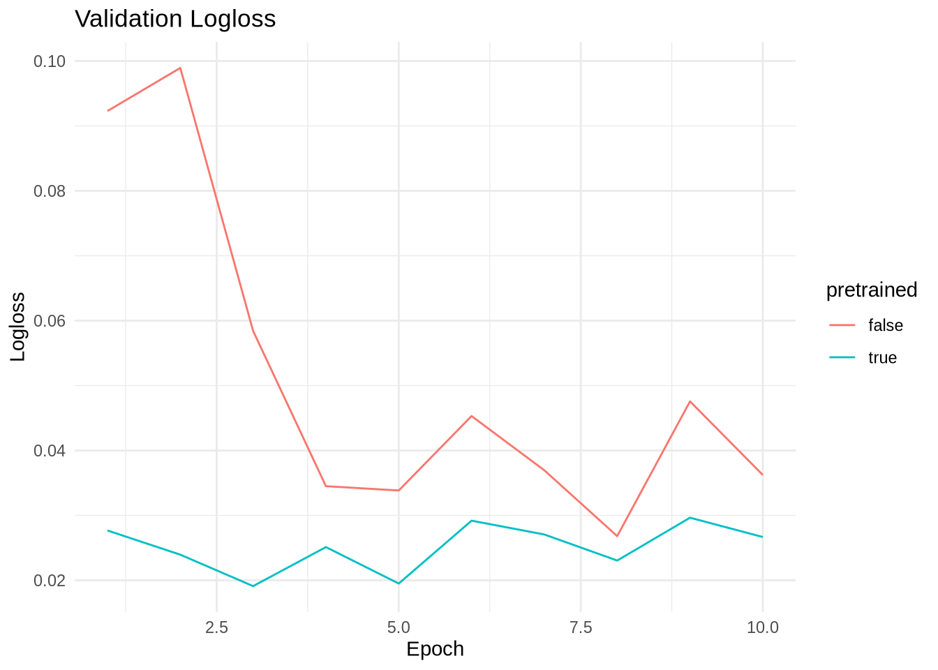
Note that when fine-tuning a pretrained model like ResNet-18, it’s possible to observe instabilities in gradients, which can manifest as fluctuating validation performance.
To address this, one can for example keep the pretrained layers fixed (for some epochs) and only train the new output head, a process known as freezing layers.
In-Context Learning
Large foundation models (such as GPT-4) even allow performing tasks on which they were not pretrained on without any finetuning. This is referred to as in-context learning or zero-shot learning. There, the task is fed into the model during inference: “Hey ChatGPT, is What is the sentiment of this sentence. Return -1 for sad, 0 for neutral, 1 for happy: