Torch Tensors

Tensors are the fundamental data structure in torch, serving as the backbone for both deep learning and scientific computing operations. While similar to R arrays, tensors offer enhanced capabilities that make them particularly suited for modern computational tasks, namely GPU acceleration and automatic differentiation (autograd).

Creating Tensors

One way to create tensors is to convert R matrices (or analogously arrays or vectors) to torch tensors using torch_tensor():

library(torch)
# From R matrices
x_matrix <- matrix(1:6, nrow = 2, ncol = 3)
x_matrix

     [,1] [,2] [,3]
[1,]    1    3    5
[2,]    2    4    6

x_tensor <- torch_tensor(x_matrix)
x_tensor

torch_tensor
 1  3  5
 2  4  6
[ CPULongType{2,3} ]

For specific types of tensors, there are also dedicated functions:

zeros_tensor <- torch_zeros(2, 3)
zeros_tensor

torch_tensor
 0  0  0
 0  0  0
[ CPUFloatType{2,3} ]

ones_tensor <- torch_ones(2, 3)
ones_tensor

torch_tensor
 1  1  1
 1  1  1
[ CPUFloatType{2,3} ]

like_tensor <- torch_zeros_like(ones_tensor)
like_tensor

torch_tensor
 0  0  0
 0  0  0
[ CPUFloatType{2,3} ]

Random Sampling

You can also randomly sample torch tensors:

normal_tensor <- torch_randn(2, 3)    # Samples from N(0,1)
uniform_tensor <- torch_rand(2, 3)    # Samples from U(0,1)

Random Seeds in torch

torch maintains its own random number generator, separate from R’s. Setting R’s random seed with set.seed() does not affect torch’s random operations. Instead, use torch_manual_seed() to control the reproducibility of torch operations.

Missing Values

Quiz: NaN vs NA

Question: What is the difference between NaN and NA in R?

Click for answer

NaN is a floating-point value that represents an undefined or unrepresentable value (such as 0 / 0).

NA is a missing value indicator used in vectors, matrices, and data frames to represent unknown or missing data.

Torch tensors do not have a corresponding representation for R’s NA values. When converting R vectors containing NAs to torch tensors, you need to be cautious:

Double: NA_real_ becomes NaN

torch_tensor(NA_real_)

torch_tensor
nan
[ CPUFloatType{1} ]

Integer: NA_integer_ becomes the smallest negative value:

torch_tensor(NA_integer_)

torch_tensor
-2.1475e+09
[ CPULongType{1} ]

Logical: NA becomes TRUE:

torch_tensor(NA)

torch_tensor
 1
[ CPUBoolType{1} ]

You should handle missing values carefully before converting them to torch tensors.

Quiz: Conversion

Question: Can you guess why the behavior is as it is?

Click for answer

When converting an R array to a torch tensors, the underlying data is simply copied over. Because R uses special values for NAs that are not standardized by the industry, torch will interprete them differently. E.g. in R, NA integers are internally represented as the smallest negative value.

In principle, torch could scan R objects for these values, but this would make conversion slower.

Tensor Properties

Shape

Like R arrays, each tensor has a shape and a dimension:

print(x_tensor$shape)

[1] 2 3

print(x_tensor$dim())

[1] 2

Data Type

Furthermore, each tensor has a datatype. Unlike base R, where typically there is one integer type (32 bits) and one floating-point type (double, 64 bits), torch differentiates between different precisions:

Floating point:

float32_tensor <- torch_ones(2, 3, dtype = torch_float32())  # Default float
float64_tensor <- torch_ones(2, 3, dtype = torch_float64())  # Double precision
float16_tensor <- torch_ones(2, 3, dtype = torch_float16())  # Half precision

Usually, you work with 32-bit floats.

Integer:

int32_tensor <- torch_ones(2, 3, dtype = torch_int32())
int64_tensor <- torch_ones(2, 3, dtype = torch_int64())  # Long
int16_tensor <- torch_ones(2, 3, dtype = torch_int16())  # Short
int8_tensor  <- torch_ones(2, 3, dtype = torch_int8())    # Byte
uint8_tensor <- torch_ones(2, 3, dtype = torch_uint8())  # Unsigned byte

Boolean:

bool_tensor <- torch_ones(2, 3, dtype = torch_bool())

You can convert between datatypes using the $to() method:

# Converting between datatypes
x <- torch_ones(2, 3)  # Default float32
x_int <- x$to(dtype = torch_int32())

Note that floats are converted to integers by truncating, not by rounding.

torch_tensor(2.999)$to(dtype = torch_int())

torch_tensor
 2
[ CPUIntType{1} ]

torch_tensor(-2.999)$to(dtype = torch_int())

torch_tensor
-2
[ CPUIntType{1} ]

Quiz: Data Types

Question: What is the advantage of 64-bit floats over 32-bit floats, what the disadvantage?

Click for answer

64-bit floats are more precise, but also require more memory. Furhermore, operations on 64-bit floats are slower than on 32-bit floats. One way to increase tensor operations is to use lower precision, a process called quantization.

Device

Each tensor lives on a “device”, where common options are:

cpu for CPU, which is available everywhere
cuda for NVIDIA GPUs
mps for Apple Silicon (M1/M2/M3) GPUs on macOS

# Create a tensor and move it to CUDA if available
x <- torch_randn(2, 3)
if (cuda_is_available()) {
  x <- x$to(device = torch_device("cuda"))
  # x <- x$cuda() also works
} else {
  print("CUDA not available; tensor remains on CPU")
}

[1] "CUDA not available; tensor remains on CPU"

print(x$device)

torch_device(type='cpu')

x <- x$to(device = "cpu")
# x <- x$cpu() also works
print(x$device)

torch_device(type='cpu')

GPU acceleration enables massive parallelization of tensor operations, often providing 10-100x speedups compared to CPU processing for large-scale computations.

Device Compatibility

Tensors must reside on the same device to perform operations between them.

Converting Tensors Back to R

You can easily convert torch tensors back to R using as_array(), as.matrix(), or $item():

0-dimensional tensors (scalars) are converted to R vectors with length 1:

{.3 .cell-code} torch_scalar_tensor(1)$item() # as_array() also works

1-dimensional tensors are converted to R vectors:

as_array(torch_randn(3))

[1] -1.4168206  0.8429176 -0.6306752

$>1$-dimensional tensors are converted to R arrays:

as_array(torch_randn(2, 2))

          [,1]       [,2]
[1,] 1.2340047  0.3126765
[2,] 0.6971866 -0.9950489

Basic Tensor Operations

Torch provides two main syntaxes for tensor operations: function-style (torch_*()) and method-style (using $).

Here’s an example with matrix multiplication:

a <- torch_tensor(matrix(1:6, nrow=2, ncol=3))
a

torch_tensor
 1  3  5
 2  4  6
[ CPULongType{2,3} ]

b <- torch_tensor(matrix(7:12, nrow=3, ncol=2))
b

torch_tensor
  7  10
  8  11
  9  12
[ CPULongType{3,2} ]

# Matrix multiplication - two equivalent ways
c1 <- torch_matmul(a, b)  # Function style
c2 <- a$matmul(b)         # Method style

torch_equal(c1, c2)

[1] TRUE

Below, there is another example using addition:

# Addition - two equivalent ways
x <- torch_ones(2, 2)
y <- torch_ones(2, 2)
z1 <- torch_add(x, y)  # Function style
z2 <- x$add(y)         # Method style

In-place Operations

Operations that modify the tensor directly are marked with an underscore suffix (_). These operations are more memory efficient as they do not allocate a new tensor:

x <- torch_ones(2, 2)
x

torch_tensor
 1  1
 1  1
[ CPUFloatType{2,2} ]

x$add_(1)  # Adds 1 to all elements in place

torch_tensor
 2  2
 2  2
[ CPUFloatType{2,2} ]

torch_tensor
 2  2
 2  2
[ CPUFloatType{2,2} ]

You can also apply common summary functions to torch tensors:

x = torch_randn(1000)
mean(x)

torch_tensor
0.0391642
[ CPUFloatType{} ]

max(x)

torch_tensor
3.31465
[ CPUFloatType{} ]

sd(x)

[1] 0.9848639

Accessing elements from a tensor is also similar to R arrays and matrices, i.e., it is 1-based.

x <- matrix(1:6, nrow = 3)
x

     [,1] [,2]
[1,]    1    4
[2,]    2    5
[3,]    3    6

xt <- torch_tensor(x)
xt

torch_tensor
 1  4
 2  5
 3  6
[ CPULongType{3,2} ]

x[1:2, 1]

[1] 1 2

xt[1:2, 1]

torch_tensor
 1
 2
[ CPULongType{2} ]

One difference between indexing torch vectors and standard R vectors is the behavior regarding negative indices. While R vectors remove the element at the specified index, torch vectors return elements from the beginning.

(1:3)[-1]

[1] 2 3

torch_tensor(1:3)[-1]

torch_tensor
3
[ CPULongType{} ]

Warning

While (R) torch is 1-based, PyTorch is 0-based. When translating PyTorch code to R, you need to be careful with this difference.

Another convenient feature in torch is the .. syntax for indexing:

arr <- array(1:24, dim = c(4, 3, 2))
arr[1:2, , ] # works

, , 1

     [,1] [,2] [,3]
[1,]    1    5    9
[2,]    2    6   10

, , 2

     [,1] [,2] [,3]
[1,]   13   17   21
[2,]   14   18   22

arr[1:2, ]    # does not work

Error in arr[1:2, ]: incorrect number of dimensions

In torch, you can achieve the same result as follows:

tensor <- torch_tensor(arr)
tensor[1:2, ..]

torch_tensor
(1,.,.) = 
   1  13
   5  17
   9  21

(2,.,.) = 
   2  14
   6  18
  10  22
[ CPULongType{2,3,2} ]

You can also specify indices after the .. operator:

tensor[.., 1]

torch_tensor
  1   5   9
  2   6  10
  3   7  11
  4   8  12
[ CPULongType{4,3} ]

Note that when you select a single element from a dimension, the dimension is removed:

dim(tensor[.., 1])

[1] 4 3

Just like in R, you can prevent this behavior by setting drop = FALSE:

dim(tensor[.., 1, drop = FALSE])

[1] 4 3 1

Tensors also support indexing by boolean masks, which will result in a 1-dimensional tensor:

tensor[tensor > 15]

torch_tensor
 17
 21
 18
 22
 19
 23
 16
 20
 24
[ CPULongType{9} ]

We can also extract the first two rows and columns of the tensor from the first index of the third dimension:

tensor[1:2, 1:2, 1]

torch_tensor
 1  5
 2  6
[ CPULongType{2,2} ]

Broadcasting Rules

Another difference between R arrays and torch tensors is how operations on tensors with different shapes are handled. For example, in R, we cannot add a matrix with shape (1, 2) to a matrix with shape (2, 3):

m1 <- matrix(1:4, nrow = 2)
m2 <- matrix(1:2, nrow = 2)
m1 + m2

Error in m1 + m2: non-conformable arrays

Broadcasting (similar to “recycling” in R) allows torch to perform operations between tensors of different shapes.

t1 <- torch_tensor(m1)
t2 <- torch_tensor(m2)
t1 + t2

torch_tensor
 2  4
 4  6
[ CPULongType{2,2} ]

There are strict rules that define when two shapes are compatible:

If tensors have a different number of dimensions, prepend 1’s to the shape of the lower-dimensional tensor until they match.
Two dimensions are compatible when:
- They are equal, or
- One of them is 1 (which will be stretched to match the other)
If any dimension pair is incompatible, broadcasting fails.

Quiz: Broadcasting Rules

Question 1: Does broadcasting work to add a tensor of shape (2, 1, 3)to a tensor of shape (4, 3)? What would be the resulting shape?

Click for answer

The resulting shape would be (2, 4, 3). Here’s why:

Prepend one to the rank of the second tensor to get (1, 4, 3).
Going dimension by dimension:
- First: 2 vs 1 -> Compatible, expand to 2
- Second: 1 vs 4 -> Compatible, expand to 4
- Third: 3 vs 3 -> Compatible, remains 3
All pairs are compatible, so broadcasting succeeds.

Question 2: Anser the same for tensors of shape (2, 3) and (3, 2)?

Click for answer

No, broadcasting would fail in this case. Here’s why:

Both tensors have the same rank (2), so no prepending is needed.
Going dimension by dimension:
- First: 2 vs 3 -> Incompatible (neither is 1)
- Second: 3 vs 2 -> Incompatible (neither is 1)
Since both dimension pairs are incompatible, broadcasting fails.

Reshaping Tensors

Torch provides several ways to reshape tensors while preserving their data:

# Create a sample tensor
x <- torch_tensor(0:15)
print(x)

torch_tensor
  0
  1
  2
  3
  4
  5
  6
  7
  8
  9
 10
 11
 12
 13
 14
 15
[ CPULongType{16} ]

We can reshape this tensor with shape (16) to a tensor with shape (4, 4).

y <- x$reshape(c(4, 4))
y

torch_tensor
  0   1   2   3
  4   5   6   7
  8   9  10  11
 12  13  14  15
[ CPULongType{4,4} ]

When x is reshaped to y, we can imagine it as initializing a new tensor of the desired shape and then filling up the rows and columns of the new tensor by iterating over the rows and columns of the old tensor:

y2 <- torch_zeros(4, 4)
for (j in 1:4) { # columns
  for (i in 1:4) { # rows
    y2[i, j] <- y[i, j]
  }
}
sum(abs(y - y2))

torch_tensor
0
[ CPUFloatType{} ]

Internally, this type of reshaping is (in many cases) implemented by changing the stride of the tensor without altering the underlying data.

x$stride()

[1] 1

y$stride()

[1] 4 1

The value of the stride indicates how many elements to skip to get to the next element along each dimension: If we move from element x[1] (1) to element x[2] (2), we move one index along the columns of y. If we move from x[1] to x[5] (5), i.e., 4 steps, we move one index along the rows of y.

This means, for example, that reshaping torch tensors can be considerably more efficient than permuting R arrays, as the latter will always allocate a new, reordered vector, while the former just changes the strides.

The functionality of strides is illustrated in the image below.

Quiz: Strides

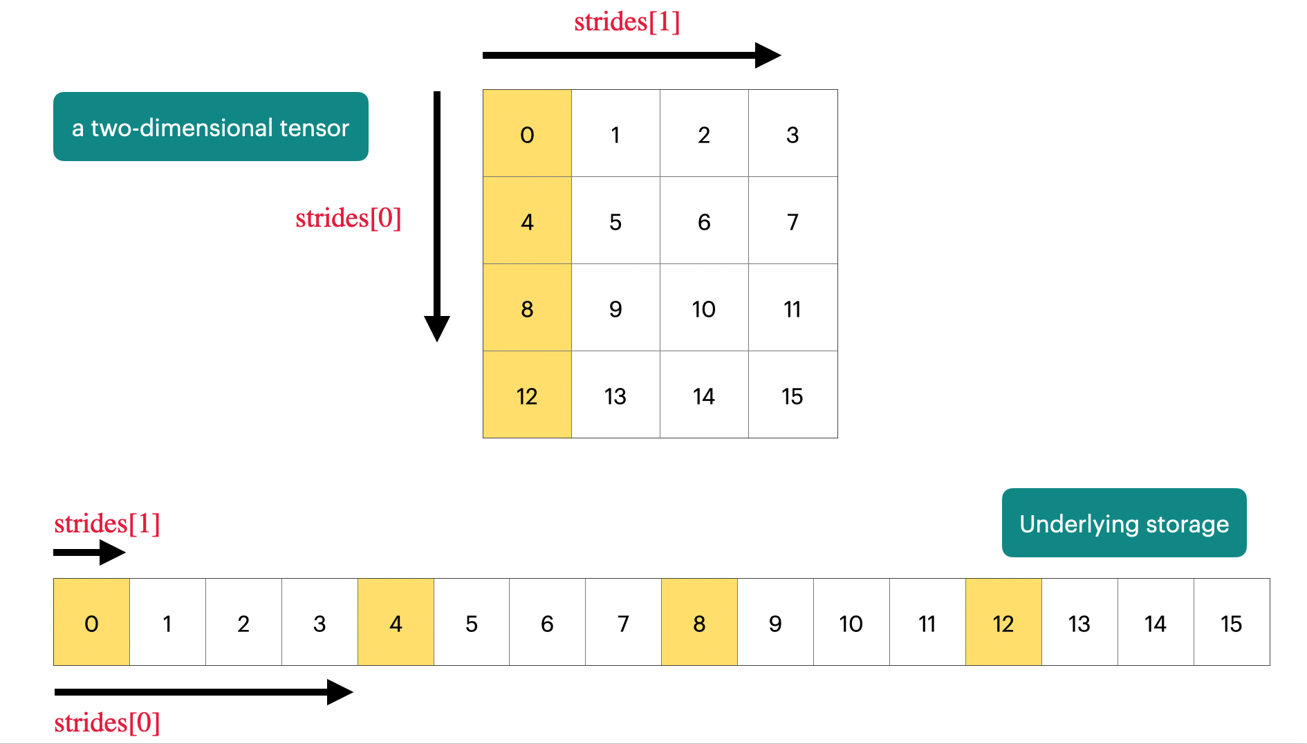
Question 1: How do you need to change the strides from a matrix with strides (4, 1) to transpose it?

Click for answer

The matrix can be transposed by changing the strides from (4, 1) to (1, 4).

y$t()$stride()

[1] 1 4

When reshaping tensors, you can also infer a dimension by setting it to -1:

x$reshape(c(-1, 4))$shape

[1] 4 4

Of course, not all reshaping operations are valid. The number of elements in the original tensor and the reshaped tensor must be the same:

x$reshape(6)

Error in (function (self, shape) : shape '[6]' is invalid for input of size 16

Reference Semantics

One key property of torch tensors is that they have reference semantics. This is different from R, where objects usually have value semantics.

x <- torch_ones(2)
y <- x
y[1] <- 5
x # was modified

torch_tensor
 5
 1
[ CPUFloatType{2} ]

This differs from R, where objects typically have value semantics:

x <- c(1, 1)
y <- x
y[1] <- 5
x # was not modified

[1] 1 1

Note

Another notable exception to values semantics are R6 classes, which are used in the mlr3 ecosystem.

When one tensor (y) shares underlying data with another tensor (x), this is called a view. It is also possible to obtain a view on a subset of a tensor, e.g., via slicing:

x <- torch_arange(1, 10)
y <- x[1:3]
y[1] <- 100
x[1]

torch_tensor
100
[ CPUFloatType{} ]

Unfortunately, similar operations might sometimes create a view and sometimes allocate a new tensor. In the example below, we create a subset that is a non-contiguous sequence, and hence a new tensor is allocated:

x <- torch_arange(1, 10)
y <- x[c(1, 3, 5)]
y[1] <- 100
x[1]

torch_tensor
1
[ CPUFloatType{} ]

If it is important to create a copy of a vector, you can call the $clone() method:

x <- torch_arange(1, 3)
y <- x$clone()
y[1] <- 10
x[1] # is still 1

torch_tensor
1
[ CPUFloatType{} ]

Warning

This is also the case for the $reshape() methods from the last section, which will in some cases create a view and in other cases allocate a new tensor with the desired shape. If you want to ensure that you create a view on a tensor, you can use the $view() method, which will fail if the required view is not possible.

Quiz: Contiguous Data

Question 1: Reshaping a 2D Tensor

Consider the tensor below:

x1 <- torch_tensor(matrix(1:6, nrow = 2, byrow = FALSE))
x1

torch_tensor
 1  3  5
 2  4  6
[ CPULongType{2,3} ]

What is the result of x1$reshape(6), i.e., what are the first, second, …, sixth elements?

Click for answer

This will result in (1, 3, 5, 2, 4, 6) because we (imagine that) first iterate over the rows and then the columns when “creating” the new tensor.