In the previous notebook, we explored how to use torch’s autograd system to fit simple linear models. We manually:
Managed the weights.
Defined the forward path for the model.
Computed gradients and updated parameters using a simple update rule: a$sub_(lr * a$grad).
For more complex models, this approach becomes cumbersome. torch offers several high-level abstractions that simplify building and training neural networks:
nn_module: A class to organize model parameters and define the forward pass, i.e. the neural network architecture.
dataset and dataloader: Classes to handle data loading and batching, replacing our manual data handling.
optim: Classes that implement various optimization algorithms, replacing our simple gradient updates.
Let’s explore how these components work together by building a neural network to classify spirals. Note that we only briefly touch on optimizers here and dedicate an additional notebook to them.
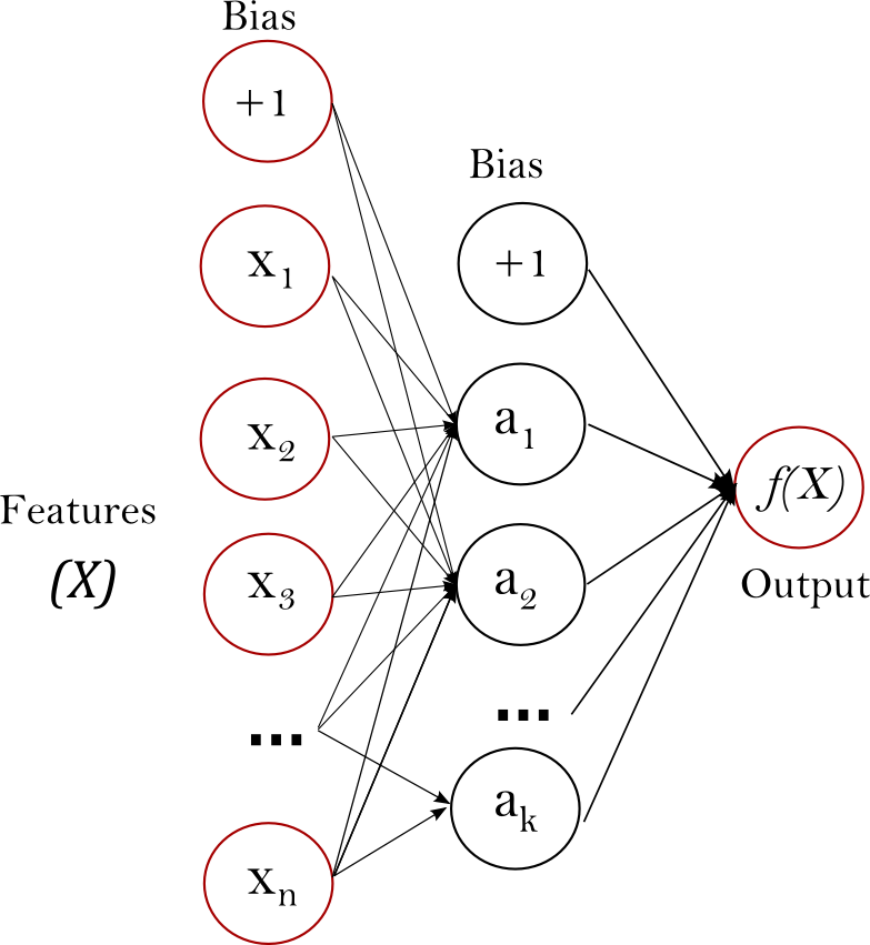
Neural Network Architecture with nn_module
The nn_module class serves several purposes, it
acts as a container for learnable parameters.
provides train/eval modes, which are essential for layers like dropout and batch normalization.
defines the forward pass of the model.
Torch offers many common neural network modules out of the box. For example, the simple linear model we created earlier (\(\hat{y} = a \times x + b\)) can be constructed using the built-in nn_linear module:
Note that while nn_modules behave like functions, they also maintain a state, primarily their parameter weights.
Implementing a custom nn_module is straightforward and requires defining two key methods:
initialize: This constructor runs when the module is created. It defines the layers and their dimensions. It can take arguments that allow to configure the network layer (such as the number of neurons in a layer).
forward: This method defines how data flows through your network: it specifies the actual computation path from inputs to outputs.
Let’s implement a simple linear regression module ourselves.
nn_simple_linear <-nn_module("nn_simple_linear",initialize =function() {# `self` refers to the object itself self$a =nn_parameter(torch_randn(1), requires_grad =TRUE) self$b =nn_parameter(torch_randn(1), requires_grad =TRUE) },forward =function(x) { self$a * x + self$b })
Note that nn_simple_linear is not an nn_module itself but an nn_module_generator. To create the nn_module, we call it, which invokes the $initialize() method defined above:
Furthermore, note that we wrapped the trainable tensors in nn_parameter(), ensuring they are included in the $parameters. Only those weights that are part of the network’s parameters (and have $requires_grad set to TRUE) will later be updated by the optimizer.
Besides parameters, neural networks can also have buffers (nn_buffer). Buffers are tensors that are part of the model’s state but don’t receive gradients during backpropagation.
Additionally, an nn_module operates in either a train or eval state that are activated by $train() and $eval() respectively.
simple_linear$train()simple_linear$training
[1] TRUE
simple_linear$eval()simple_linear$training
[1] FALSE
Some nn_modules (such as batch normalization) behave differently depending on this mode, so it’s essential to ensure that the network is in the correct mode.
Another important method of a network is $state_dict(), which returns the network’s parameters and buffers.
The state dict can, for example, be used to save the network’s weights for later use. Note that, in general, you cannot simply save and load torch objects using saveRDS and readRDS:
Besides adding parameters and buffers to the network’s state dict by registering nn_parameters and nn_buffers in the module’s $initialize() method, you can also register other nn_modules, which we will do in the next section.
The World is Not Linear
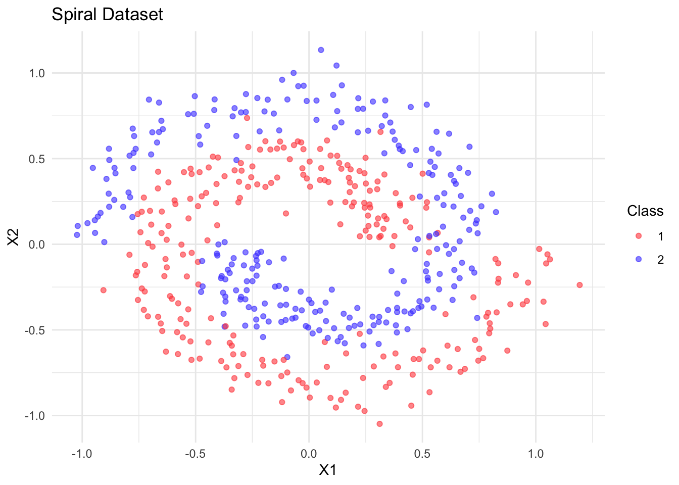
While we have so far explained much of torch’s functionality using simple linear networks, the main idea of deep learning is to model complex, non-linear relationships. Below, we generate some non-linear synthetic spiral data for binary classification:
library(torch)library(ggplot2)library(mlbench)# Generate spiral dataset.seed(123)n <-500spiral <-mlbench.spirals(n, sd =0.1)# Convert to data framespiral_data <-data.frame(x1 = spiral$x[,1],x2 = spiral$x[,2],label =as.factor(spiral$classes))
The data looks like this:
While linear models are often useful and have helped us explain the torch API, they are limited in capturing the complex, non-linear patterns commonly present in real-world data, especially unstructured types like images, text, audio, and video. Deep neural networks typically consist of many different layers (hence the name “deep”) and combine linear and non-linear layers with various other components, allowing them to represent highly complex functions. Traditional machine learning and statistics rely on manual feature engineering to transform raw inputs, whereas deep neural networks have revolutionized this process by automatically learning hierarchical features directly from the data.
One challenging problem is defining a neural network architecture for a given task. This is where architectural choices and their associated inductive biases come into play. An inductive bias represents a set of structural assumptions of how our predictive function looks like and behaves. These biases help the model generalize beyond its training data by favoring certain solutions over others.
Some examples of inductive biases in different neural network architectures are convolutional neural networks, transformers, and multi-layer perceptrons (MLPs). Here, we will focus on MLPs, which are the most basic type of neural network (but are an integral part of basically every other neural network).
The different layers in a Multi-Layer Perceptron (MLP) consist of an affine-linear transformation followed by a non-linear function, such as a ReLU activation function:
Our simple multi-layer perceptron has minimal inductive biases:
Continuity: Similar inputs should produce similar outputs.
Hierarchical Feature Learning: Each layer builds increasingly abstract representations.
This flexibility makes MLPs general-purpose learners, but they may require more data or parameters to learn patterns that specialized architectures can discover more efficiently.
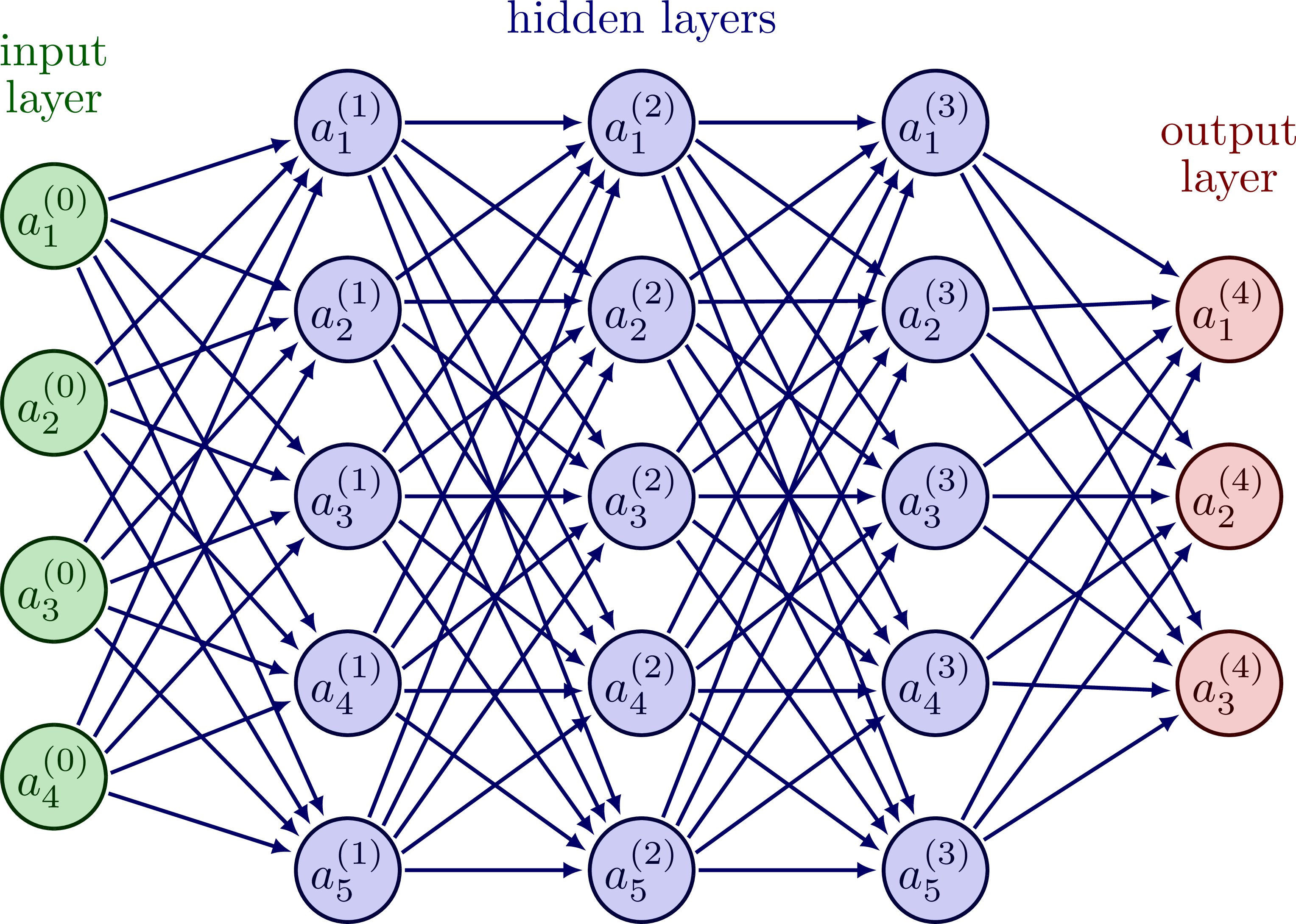
For our spirals classification problem, we will use a simple MLP with three hidden layers:
Instead of creating an nn_relu() during network initialization, we could have used the nnf_relu function directly in the forward pass. This is possible for activation functions as they have no trainable weights.
In general, nn_ functions create module instances that can maintain state (like trainable weights or running statistics), while nnf_ functions provide the same operations as pure functions without any state.
Furthermore, for simple sequential networks, we could have used nn_sequential to define the network instead of nn_module. This allows you to chain layers together in a linear fashion without explicitly defining the forward pass.
The architecture of such an MLP layer is visualized below:
At this point, let’s briefly discuss the ‘head’ of the network, as well as loss functions.
Classification
The output dimension of a classification network is usually the number of classes, which is 2 in our case. However, the output is not probabilities but logit scores. To convert a vector of scores to probabilities, we apply the softmax function:
The most commonly used loss function is cross-entropy. For a true probability vector \(p\) and a predicted probability vector \(q\), the cross-entropy is defined as:
\[ \text{CE}(p, q) = - \sum_i p_i \log(q_i) \]
Note that when the true probability \(p\) is 1 for the true class and 0 for all other classes, the cross-entropy simplifies to:
\[ \text{CE}(p, q) = - \log(q_{y}) \]
where \(y\) is the true class and \(q_y\) is its predicted probability.
To calculate the cross-entropy loss, we need to pass the predicted scores and the true class indices to the loss function. The classes should be labeled from 1 to C for a total of C classes.
For regression tasks, the final layer is almost always a simple linear layer with a single output. We can construct a version of the spiral network for regression by changing the final layer to a linear layer with a single output:
Finally, it’s important to note that there is nothing inherently ‘magical’ about nn_modules. We could have equally implemented the same network manually ourselves, i.e. without using the nn_module class.
Dataset and DataLoader
Besides the network architecture, another essential component of deep learning is the dataset. The two central classes are dataset and dataloader, which address separate concerns:
dataset: Handles data storage and access to individual samples. The methods are:
.getitem(): Returns a single sample, regardless of the retrieval method (e.g., reading from disk or fetching from a database).
.getbatch() (optional): Returns a full batch.
.length(): Returns the dataset size.
dataloader: Given a dataset, handles batching, shuffling, and parallel loading.
We will start by creating a custom dataset class for the spiral problem. In its $initialize() method, it expects a data.frame with columns "x1", "x2", and "label". We then convert these to tensors and store them in the object.
Below, we implement .getitem(), but we could also implement .getbatch(), which retrieves a vector of indices. Note that implementing .getbatch() can sometimes offer performance benefits.
train_loader <-dataloader( train_dataset,batch_size =64,# shuffling is important when your data is orderedshuffle =TRUE,drop_last =FALSE)valid_loader <-dataloader( valid_dataset,batch_size =64,shuffle =FALSE,drop_last =FALSE)
The most common way to iterate over the batches of a dataloader is to use the coro::loop function, which resembles a for loop:
n_batches <-0coro::loop(for (batch in train_loader) {# do something with the batch n_batches <- n_batches +1})print(n_batches)
[1] 7
It is also possible to manually iterate over the batches by first creating an iterator using torch::dataloader_make_iter() and then calling dataloader_next() until NULL is returned, indicating that the iterator is exhausted.
iter <-dataloader_make_iter(train_loader)n_batches <-0while (!is.null(batch <<-dataloader_next(iter))) { n_batches <- n_batches +1}print(n_batches)
[1] 7
The torch::dataloader class also has other parameters that e.g. allow to parallelize the loading. This will be covered in the Training Efficiency notebook.
Training Loop
To train our MLP on the data, we need to specify how the gradients will update the network parameters, which is the role of the optimizer. While we’ll cover more complex optimizers in the next section, we’ll use a vanilla SGD optimizer with a learning rate of 0.3 and pass it the parameters of the model we wish to optimize. Note that it is important to move the model to the correct device before passing it to the optimizer.
# Move model to devicedevice <-if (cuda_is_available()) "cuda"else"cpu"model$to(device = device)optimizer <-optim_sgd(model$parameters, lr =0.3)
For the training loop, we only need methods from the optimizer class:
The $step() method updates the weights based on the gradients and the optimizer configuration (e.g., the learning rate).
The $zero_grad() method sets the gradients of all parameters handled by the optimizer to 0.
Now, let’s put everything together:
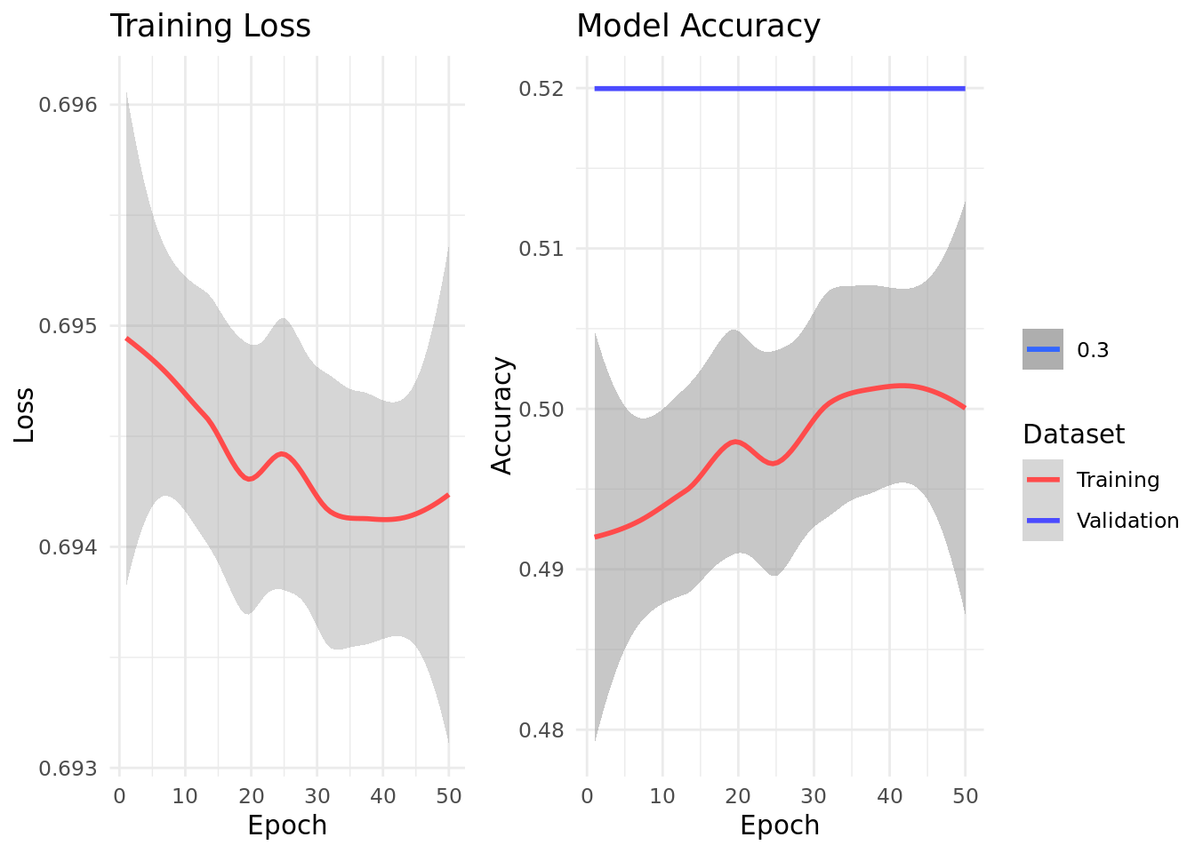
# Training settingsn_epochs <-50# Training loophistory <-list(loss =numeric(), train_acc =numeric(), valid_acc =numeric())for(epoch inseq_len(n_epochs)) { model$train() # Set to training mode# Training loop train_losses <-numeric() train_accs <-numeric() coro::loop(for(batch in train_loader) {# Move batch to device x <- batch$x$to(device = device) y <- batch$y$to(device = device)# Forward pass and average loss computation output <-model(x) loss <-nnf_cross_entropy(output, y)# Backward pass optimizer$zero_grad() loss$backward()# Update parameters optimizer$step()# Store training losses train_losses <-c(train_losses, loss$item()) train_accs <-c(train_accs, mean(as_array(output$argmax(dim =2) == y))) }) history$loss <-c(history$loss, mean(train_losses)) history$train_acc <-c(history$train_acc, mean(train_accs))# Validation loop# Set model to evaluation mode model$eval() valid_accs <-numeric() coro::loop(for(batch in valid_loader) { x <- batch$x$to(device = device) y <- batch$y$to(device = device)# IMPORTANT: Disable gradient tracking output <-with_no_grad(model(x)) valid_acc <-as_array(output$argmax(dim =2) == y) valid_accs =c(valid_accs, mean(valid_acc)) }) history$valid_acc <-c(history$valid_acc, mean(valid_accs))}
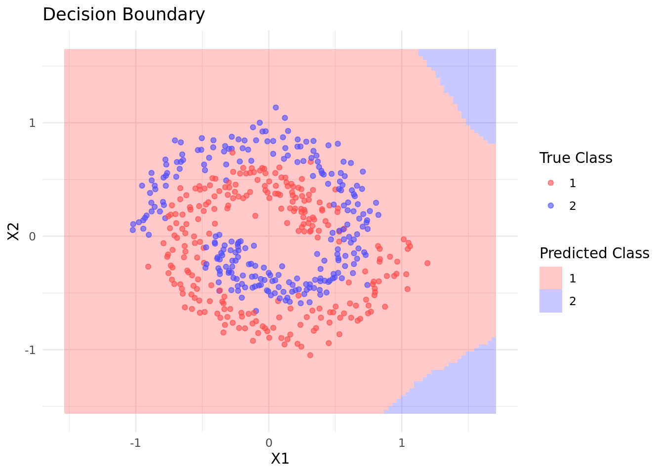
The decision boundary plot shows how our neural network learned to separate the spiral classes, demonstrating its ability to learn non-linear patterns that a simple linear model couldn’t capture.
We can also visualize the predictions of our final network:
This example demonstrates how torch’s high-level components work together to build and train neural networks:
nn_module manages our parameters and network architecture.
The optimizer handles parameter updates.
The dataset and dataloader classes work in tandem for data loading.
The training loop integrates everything seamlessly.