library(torch)

a <- torch_tensor(2, requires_grad = TRUE)
a$requires_grad
[1] TRUEb <- torch_tensor(1, requires_grad = TRUE)
x <- torch_tensor(3)Automatic differentiation (autograd) is one of torch’s key features, enabling the automatic computation of gradients for optimization tasks like training neural networks. Unlike numerical differentiation, which approximates gradients using finite differences, autograd computes exact gradients by tracking operations as they are performed and automatically applying the chain rule of calculus. This makes it possible to efficiently compute gradients of complex functions with respect to many parameters — a critical requirement for training modern neural networks.
Autograd works by building a dynamic computational graph of operations, where each node represents a tensor and each edge represents a mathematical operation.
Why do we need automatic differentiation?
In deep learning, training a model requires iteratively updating parameters to minimize a loss function, which measures the difference between predictions and actual data. These updates depend on calculating gradients of the loss with respect to model parameters, information used by optimization algorithms like stochastic gradient descent (SGD). Automatic Differentiation eliminates the need to manually derive these gradients.
To use autograd, tensors must have their requires_grad field set to TRUE. This can either be set during tensor construction or changed afterward using the in-place modifier $requires_grad_(TRUE). In the context of deep learning, we track the gradients of the weights of a neural network. The simplest “neural network” is a linear model with slope \(a\) and bias \(b\) and a single input \(x\).
The forward pass is defined as:
\[\hat{y} = u + b = a \times x + b\]
We might be interested in how the prediction \(\hat{y}\) changes for the given \(x\) when we change the weight \(a\) or the bias \(b\). We will later use this to adjust the weights \(a\) and \(b\) to improve predictions, i.e., to perform gradient-based optimization. To write down the gradients, let \(u = a \times x\) denote the intermediate tensor from the linear predictor.
We can now derive the gradients for:
Weight \(a\):
This is expressed by the gradient \(\frac{\partial \hat{y}}{\partial a}\). We can compute the derivative using the chain rule as:
\[\frac{\partial \hat{y}}{\partial a} = \frac{\partial \hat{y}}{\partial u} \cdot \frac{\partial u}{\partial a} = 1 \cdot x = x\]
Bias \(b\):
\[\frac{\partial \hat{y}}{\partial b} = 1\]
library(torch)
a <- torch_tensor(2, requires_grad = TRUE)
a$requires_grad[1] TRUEb <- torch_tensor(1, requires_grad = TRUE)
x <- torch_tensor(3)We can use the weights and input to perform a forward pass:
u <- a * x
y_hat <- u + b
When you perform operations on tensors with gradient tracking, torch builds a computational graph on the fly. In the figure below:
graph TD
    a[a] --> mul[Multiply]
    x[x] --> mul
    mul --> u[u]
    u --> add[Add]
    b[b] --> add
    add --> y_hat[y_hat]

    %% Styling
    classDef input fill:#a8d5ff,stroke:#333
    classDef op fill:#ffe5a8,stroke:#333
    classDef output fill:#a8ffb6,stroke:#333
    classDef grad fill:#ffa8a8,stroke:#333,stroke-dasharray:5,5
    classDef intermediate fill:#d5a8ff,stroke:#333
    classDef nograd fill:#e8e8e8,stroke:#333

    class a,b input
    class mul,add op
    class y_hat output
    class u intermediate
    class x nograd
Each tensor that is a function output knows how to calculate gradients with respect to its inputs.
y_hat$grad_fnAddBackward0u$grad_fnMulBackward0To calculate the gradients \(\frac{\partial \hat{y}}{\partial a}\) and \(\frac{\partial \hat{y}}{\partial b}\), we can traverse this computational graph backwards, invoke the differentiation functions, and multiply the individual derivatives according to the chain rule.
In torch, this is done by calling $backward() on y_hat. Note that $backward() can only be called on scalar tensors. Afterwards, the gradients are accessible in the $grad field of the tensors a and b:
# Compute gradients
y_hat$backward()

# Access gradients
print(a$grad)  # dy/da = x = 3
torch_tensor
3
[ CPUFloatType{1} ]print(b$grad) # dy/db = 1torch_tensor
1
[ CPUFloatType{1} ]Note that for the intermediate value u, no gradient is stored.
When you want to perform an operation on tensors that require gradients without tracking this specific operation, you can use the context manager with_no_grad({...}).
In the next section, we will show how we can use gradients to train our simple linear model.
We can use autograd to fit a simple linear regression model. Let’s first generate some synthetic observations \(\{(x^{(i)}, y^{(i)})\}_{i = 1}^n\).
library(ggplot2)

# Set random seed for reproducibility
torch_manual_seed(42)

# Generate synthetic data
n <- 100
a_true <- 2.5
b_true <- 1.0

# Create input X and add noise to output Y
X <- torch_randn(n)
noise <- torch_randn(n) * 0.5
Y <- X * a_true + b_true + noise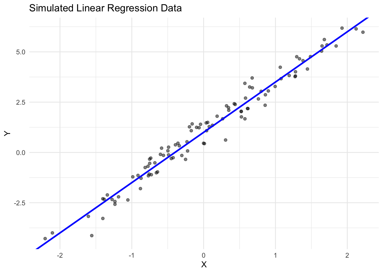
To start the optimization, we need to randomly initialize our parameters a and b.
a <- torch_randn(1, requires_grad = TRUE)
b <- torch_randn(1, requires_grad = TRUE)
To optimize the parameters \(a\) and \(b\), we further need to define the loss function that quantifies the discrepancy between our predictions \(\hat{y}\) and the observed values \(y\). The standard loss for linear regression is the L2 loss:
\[ \mathcal{L}(y, \hat{y}) = (y - \hat{y})^2\]
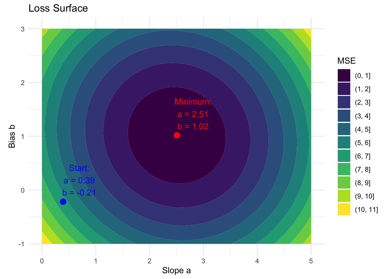
This allows us to define the empirical risk function that assigns the average loss over all observations to a given pair of parameters \(a\) and \(b\):
\[ \hat{\mathcal{R}}(a, b) = \frac{1}{n} \sum_{i=1}^n (y^{(i)} - (a \times x^{(i)} + b))^2\]
This risk function is visualized in the contour plot below.
We can optimize the parameters \(a\) and \(b\) to converge to the minimum by using gradient descent. Gradient descent is a fundamental optimization algorithm that helps us find the minimum of a function by iteratively moving in the direction of steepest descent.
The gradient of a function points in the direction of the steepest increase—like pointing uphill on mountainous terrain. Therefore, the negative gradient points in the direction of the steepest decrease—like pointing downhill.
Gradient descent uses this property to iteratively:
Note that the gradient only tells us in which direction we have to go, not how far. The length of the step should not be:
The general update formula for the weights \(a\) and \(b\) is:
\[a_{t+1} = a_t - \eta \frac{\partial \hat{R}}{\partial a_t}\] \[b_{t+1} = b_t - \eta \frac{\partial \hat{R}}{\partial b_t}\]
where \(\eta\) is the learning rate / step size, and \(\hat{R}\) is the empirical risk function.
In practice, when dealing with large datasets, computing the gradient over the entire dataset can be computationally expensive. Instead, we often use Stochastic Gradient Descent (SGD), where the gradient is estimated using only a few observations (a so called ‘batch’), but more details on that will be given later.
We start by implementing a single stochastic gradient step. Note that if we repeatedly call loss$backward(), the gradients in a and b would accumulate, so we set them to 0 after performing the update. The return value of the update function are the parameter values and the loss so we can plot them later. Also, note that we mutate the parameters a and b in-place (suffix _).
update_params <- function(X_batch, Y_batch, lr, a, b) {
  # Perform forward pass, calculate average loss
  Y_hat <- X_batch * a + b
  loss <- mean((Y_hat - Y_batch)^2)

  # Calculate gradients
  loss$backward()

  # We don't want to track gradients when we update the parameters.
  with_no_grad({
    a$sub_(lr * a$grad)
    b$sub_(lr * b$grad)
  })

  # Ensure gradients are zero
  a$grad$zero_()
  b$grad$zero_()

  # $item() converts scalar tensors to R vectors of length 1
  list(
    a = a$item(),
    b = b$item(),
    loss = loss$item()
  )
}
Next, we use this function to learn the parameters \(a\) and \(b\) by repeatedly applying the update function.
library(data.table)
# Hyperparameters
lr <- 0.02
epochs <- 10
batch_size <- 10
# Split data into 10 batches of size 10
batches <- split(sample(1:100), rep(seq_len(batch_size), length.out = 100))
history <- list()
for (epoch in seq_len(epochs)) {
for (step in 1:10) {
result <- update_params(X[batches[[step]]], Y[batches[[step]]], lr, a, b)
history <- append(history, list(as.data.table(result)))
}
}
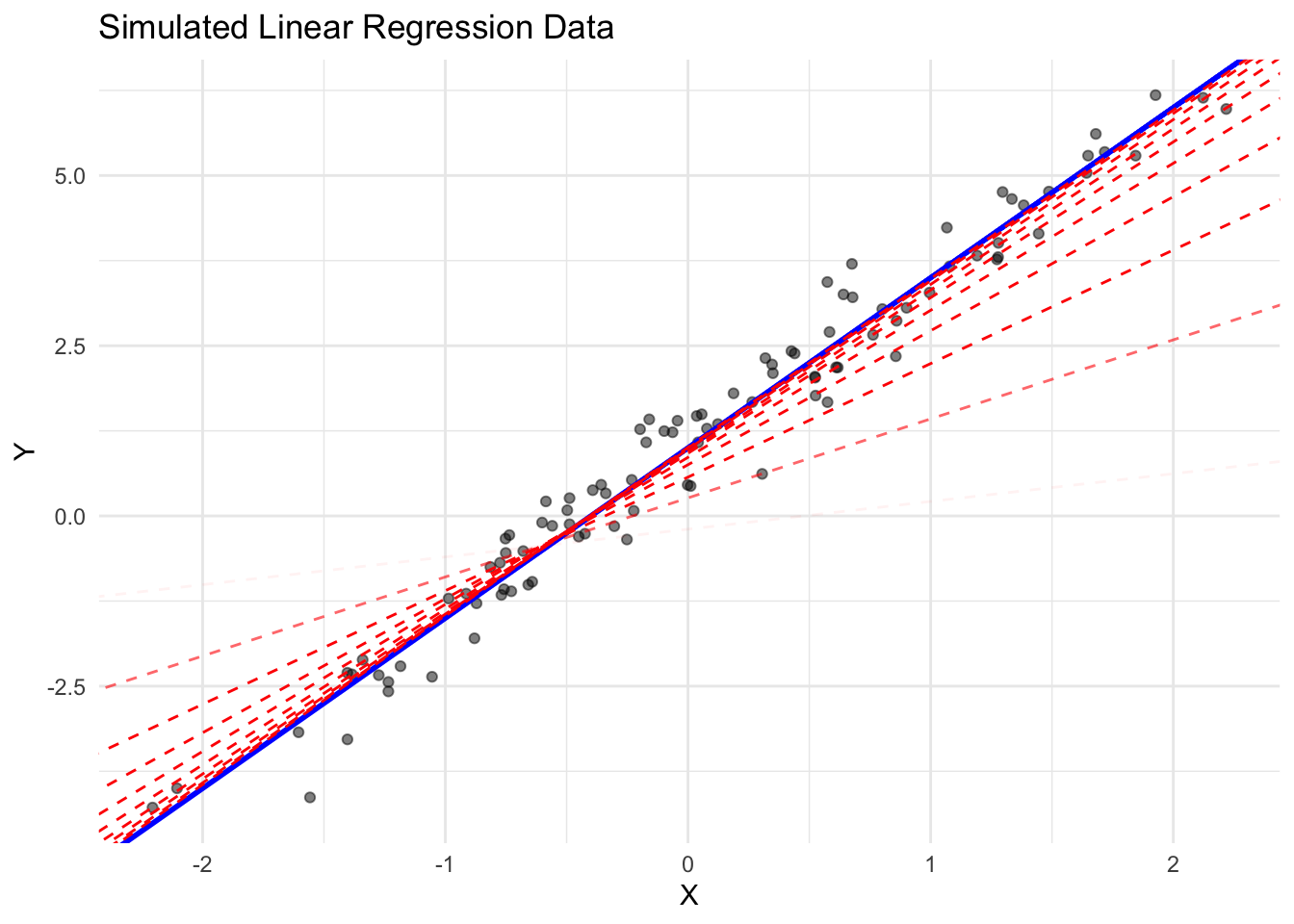
history = rbindlist(history)This example demonstrates how we can use torch’s autograd to implement stochastic gradient descent for fitting a simple linear regression model. The dashed red lines show the progression of the model during training, with increasing opacity for later steps. The blue line represents the true relationship.
We can also visualize the parameter updates over time embedded in the empirical risk landscape:
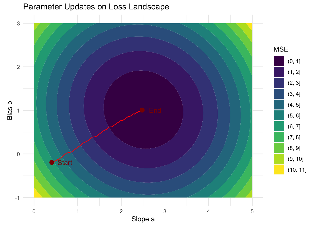
Of course, better solutions exist for estimating a simple linear model. Because the risk is simply a quadratic function, we can analytically solve this optimization problem by solving the normal equations. The motivation behind the example was merely to demonstrate how we can utilize an autograd system to estimate the parameters of a model.